Scikit Image - Morphological Reconstruction of an Image

---

---

Morphological reconstruction is a fundamental concept in image processing and computer vision tasks. It is used to enhance or manipulate certain features in an image by combining two images: a "seed" image and a "mask" image. These two images interact to create a new image, which can have specific properties depending on the reconstruction process applied (dilation or erosion). This technique is often used for tasks such as noise reduction, feature enhancement, segmentation, and more.

The scikit library provides a function called reconstruction() in the morphology module to perform the morphological reconstruction of an image.

Using the skimage.morphology.reconstruction() function

The morphology.reconstruction() function is used to perform the morphological reconstruction of an image using either dilation or erosion methods.

Morphological reconstruction by dilation is similar to basic dilation: it replaces low-intensity values with high-intensity values. However, basic dilation uses a footprint to decide how far the value can spread in the input image. In contrast, reconstruction involves two images: a "seed" image that specifies the spreading values and a "mask" image that sets the maximum allowed value for each pixel. The mask image, like the footprint, constrains the spread of high-intensity values.

Reconstruction by erosion is simply the inverse: low-intensity values expand from the seed image but are restricted by the mask image, representing the minimum allowed value.

Another way to view reconstruction is as a method to separate connected regions in an image. For dilation, it links regions marked by local maxima in the seed image: nearby pixels less than or equal to these maxima become part of the connected region. Local maxima with values greater than the seed image will be limited to the seed value.

Syntax

Following is the syntax of this function −

skimage.morphology.reconstruction(seed, mask, method='dilation', footprint=None, offset=None)

Parameters

• Seed (ndarray): The seed image, indicates values that are dilated or eroded.
• Mask (ndarray): The maximum (dilation) or minimum (erosion) values are allowed at each pixel.
• Method {dilation|erosion}, optional: it allows you to choose reconstruction between 'dilation' or 'erosion'. The default is 'dilation'.
• Footprint (ndarray): An optional neighborhood definition, typically a square or cube. Default is the n-D square of radius equal to 1 (i.e. a 3x3 square for 2D images, a 3x3x3 cube for 3D images, etc.).
• Offset (ndarray): An optional parameter specifies the coordinates of the center of the footprint. The default is the geometrical center of the footprint.

Return Value

It returns the reconstructed ndarray, which is the result of the morphological reconstruction process.

Example

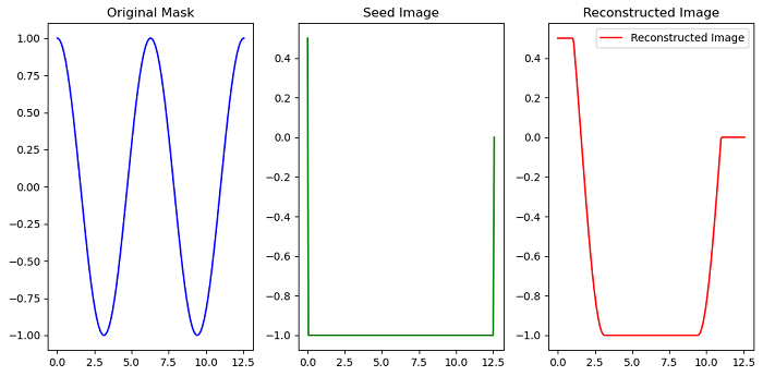
The following example demonstrates how morphological reconstruction by dilation can be used to manipulate and limit the spread of intensity values.

import numpy as np
from skimage.morphology import reconstruction
import matplotlib.pyplot as plt

# Create a simple image with peaks
x = np.linspace(0, 4 * np.pi, 200)
y_mask = np.cos(x)

# Create a seed image
y_seed = y_mask.min() * np.ones_like(x)
y_seed[0] = 0.5 
y_seed[-1] = 0  

# Perform morphological reconstruction by dilation 
y_rec = reconstruction(y_seed, y_mask)

# Plot the original mask, seed, and reconstructed image
plt.figure(figsize=(10, 5))
plt.subplot(131)
plt.plot(x, y_mask, 'b', label='Original Mask')
plt.title('Original Mask')

plt.subplot(132)
plt.plot(x, y_seed, 'g', label='Seed Image')
plt.title('Seed Image')

plt.subplot(133)
plt.plot(x, y_rec, 'r', label='Reconstructed Image')
plt.title('Reconstructed Image')

plt.legend()
plt.tight_layout()
plt.show()

Output

On executing the above program, you will get the following output −

Example

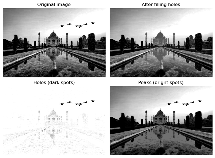
This example will perform the hole-filling and peak detection of an image using the morphological reconstruction() function.

import matplotlib.pyplot as plt
import numpy as np
from skimage import io, exposure, morphology

# Load an image
image = io.imread('Images/Blue.jpg')

# Preprocess the image to enhance features
image = exposure.rescale_intensity(image, in_range=(50, 200))

# Fill Holes (using the erosion method)
seed_fill = np.copy(image)
seed_fill[1:-1, 1:-1] = image.max()
mask_fill = image
filled_image = morphology.reconstruction(seed_fill, mask_fill, method='erosion')

# Find Peaks (using the dilation method)
seed_peak = np.copy(image)
seed_peak[1:-1, 1:-1] = image.min()
mask_peak = image
peaks_image = morphology.reconstruction(seed_peak, mask_peak, method='dilation')

# Plot the results
fig, ax = plt.subplots(2, 2, figsize=(8, 6), sharex=True, sharey=True)
ax = ax.ravel()

ax[0].imshow(image, cmap='gray')
ax[0].set_title('Original image')
ax[0].axis('off')

ax[1].imshow(filled_image, cmap='gray')
ax[1].set_title('After filling holes')
ax[1].axis('off')

ax[2].imshow(image - filled_image, cmap='gray')
ax[2].set_title('Holes (dark spots)')
ax[2].axis('off')

ax[3].imshow(peaks_image, cmap='gray')
ax[3].set_title('Peaks (bright spots)')
ax[3].axis('off')

plt.tight_layout()
plt.show()

Output

On executing the above program, you will get the following output −