Scikit Image - Conversion to luv colorspace

---

---

The Luv color space also referred to as CIELUV, is a color space defined by the International Commission on Illumination (abbreviated CIE) in 1976. It is a transformation of the CIE XYZ color space and is designed to achieve perceptual uniformity. It is commonly used in various applications, including computer graphics and color-related tasks in image processing.

In the scikit-image library, you can use the CIELUV color space through the color.rgb2luv() and color.xyz2luv() functions. These functions allow you to convert images in the RGB, and XYZ color spaces to the CIELUV color space.

Converting RGB image to CIE-Luv color space

The skimage.color.rgb2luv() method performs the conversion from the RGB (Red, Green, Blue) color space to the CIE-Luv color space.

Syntax

Following is the syntax of this function −

skimage.rgb2luv(rgb, *, channel_axis=-1)

Parameters

• rgb: It is an array-like object representing the image in RGB format. The shape of the array should be at least 2-D with the last dimension having a size of 3, representing the three channels (Red, Green, and Blue).
• channel_axis: An optional parameter indicating which axis of the array corresponds to channels. By default, it is set to -1, which corresponds to the last axis. This parameter was introduced in scikit-image new version 0.19.

Return Value

The method returns a ndarray representing the output image in CIE Luv format. And the dimensions of the output array are the same as the input array.

Exception

And the method will raise the ValueError. If the rgb input is not at least 2-D with a shape of (..., 3, ...), indicating the presence of the three channels.

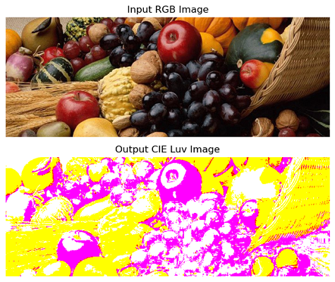
Example

The following example demonstrates the conversion of an image in RGB color space to CIE Luv color space using color.rgb2luv() method.

import numpy as np
from skimage import color, io
import matplotlib.pyplot as plt

# Read an RGB image
rgb_image = io.imread('Images/Fruits.jpg')

# Convert RGB to CIE Luv 
luv_image = color.rgb2luv(lab_image)

# Display the RGB and luv images using Matplotlib
fig, axes = plt.subplots(nrows=2, ncols=1, figsize=(10, 5))

axes[0].imshow(rgb_image)
axes[0].set_title('Input RGB Image')
axes[0].axis('off')

axes[1].imshow(luv_image)
axes[1].set_title('Output CIE Luv Image')
axes[1].axis('off')

plt.tight_layout()
plt.show()

Output

When you run the above program, it will generate the following output −

Converting XYZ image to CIE-Luv color space

The skimage.color.xyz2luv() method performs the conversion from the XYZ color space to the CIE-Luv color space.

Syntax

Following is the syntax of this function −

skimage.xyz2luv(xyz, illuminant='D65', observer='2', *, channel_axis=-1)

Parameters

• xyz (array_like): The input image array in XYZ format. The shape of the array should be at least 2-D with the last dimension having a size of 3, representing the three channels (X, Y, and Z).
• illuminant: it is an optional string parameter representing the name of the illuminant {A, B, C, D50, D55, D65, D75, E}. The default value is 'D65'.
• observer: An optional string parameter representing the aperture angle of the observer {2, 10, R}. The default value is '2'.
• channel_axis: An optional parameter indicating which axis of the array corresponds to channels. By default, it is set to -1, which corresponds to the last axis. This parameter was introduced in scikit-image new version 0.19.

Return Value

The method returns a ndarray representing the output image in CIE Luv format. And the dimensions of the output array are the same as the input array.

Exception

And the method will raise the ValueError if −

• The xyz input is not at least 2-D with a shape of (..., 3, ...), indicating the presence of the three channels.
• Or, either the illuminant or the observer angle is unsupported or unknown.

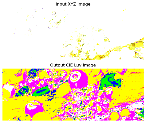
Example

The following example demonstrates the conversion of an image in XYZ color space to CIE Luv color space using color.xyz2luv() method.

import numpy as np
from skimage import color, io
import matplotlib.pyplot as plt

# Read an RGB image
rgb_image = io.imread('Images/Fruits.jpg')

# Convert RGB to XYZ format
xyz_image = color.rgb2xyz(lab_image)

# Finally convert XYZ to CIE Luv  format
luv_image = color.xyz2luv(lab_image)

# Display the RGB and luv images using Matplotlib
fig, axes = plt.subplots(nrows=2, ncols=1, figsize=(10, 5))

axes[0].imshow(xyz_image)
axes[0].set_title('Input XYZ Image')
axes[0].axis('off')

axes[1].imshow(luv_image)
axes[1].set_title('Output CIE Luv Image')
axes[1].axis('off')

plt.tight_layout()
plt.show()

Output