Scikit Image - Harris Corner Detection

Quiz

The Harris corner detection is a widely used corner detection operator in computer vision. It was developed by Chris Harris and Mike Stephens in 1988 as an improvement over Moravec's corner detector. The Harris corner detector considers the differential of the corner score concerning direction directly, instead of employing shifting patches for various 45-degree angles. This approach leads to improved accuracy in distinguishing between edges and corners.

This detector has been subsequently enhanced and integrated into various computer vision applications to preprocess images for further processing, making it a valuable tool for feature extraction and image analysis.

The scikit image library offers the corner_harris function within its feature module, allowing users to apply the Harris corner detector to images.

Using the skimage.feature.corner_harris() function

The corner_harris() function is used to compute a Harris corner measure response image.

This corner detector uses information from the auto-correlation matrix A, which is computed as follows −

$$\mathrm{A= \begin{matrix} [(imx^{\ast \ast}2)(imx^{\ast}imy)] = [Axx \: Axy] \\ [(imx^{\ast}imy)(imy{\ast \ast}2)] [Axy \: Ayy] \end{matrix}}$$

Where imx and imy are the first derivatives of the image, typically averaged with a Gaussian filter. This matrix A characterizes the local image structure.

$$\mathrm{det(A)-k^{\ast} trace(A)^{\ast \ast} 2}$$

$$\mathrm{2^{\ast}det(A)/(trace(A)+eps)}$$

Syntax

Following is the syntax of the function −

skimage.feature.corner_harris(image, method='k', k=0.05, eps=1e-06, sigma=1)

image (M, N) ndarray: The input image on which the Harris corner detection is performed.
method (optional): Specifies the method used to compute the response image from the auto-correlation matrix. The available options are: 'k' or 'eps'.
k (optional): A float representing the sensitivity factor to separate corners from edges, typically in range [0, 0.2]. Small values of k result in detection of sharp corners. (used if method is 'k').
eps (optional): A float representing the normalization factor (Noble's corner measure).
sigma (optional): The standard deviation used for the Gaussian kernel, which serves as a weighting function for the auto-correlation matrix.

The function returns a response ndarray, which is the Harris response image.

Example

The following example demonstrates how to use the Harris corner detector to identify corner-like features in a simple binary image and then detect and display the coordinates of these corners using the corner_peaks function.

import numpy as np
from skimage.feature import corner_harris, corner_peaks

# Create a 10x10 image with a square-shaped region
square = np.zeros([10, 10])
square[2:8, 2:8] = 1

# Convert the image to integers
square = square.astype(int)

# Compute the Harris corner response
corner_response = corner_harris(square)

# Find and mark the corner peaks with a minimum distance of 1 pixel
corners = corner_peaks(corner_response, min_distance=1)

# Display the input and output arrays
print("The Original array:", square)
print('The corner points on the response array:', corners)

Output

The Original array: 
[[0 0 0 0 0 0 0 0 0 0]
 [0 0 0 0 0 0 0 0 0 0]
 [0 0 1 1 1 1 1 1 0 0]
 [0 0 1 1 1 1 1 1 0 0]
 [0 0 1 1 1 1 1 1 0 0]
 [0 0 1 1 1 1 1 1 0 0]
 [0 0 1 1 1 1 1 1 0 0]
 [0 0 1 1 1 1 1 1 0 0]
 [0 0 0 0 0 0 0 0 0 0]
 [0 0 0 0 0 0 0 0 0 0]]

The corner points on the response array: 
[[2 2]
 [2 7]
 [7 2]
 [7 7]]

Example

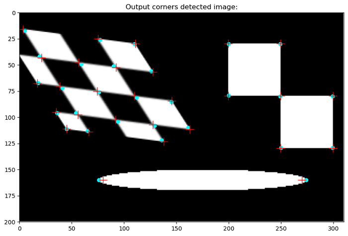
Here's an example that demonstrates the application of the Harris corner detection algorithm (corner_harris) to identify corner-like features within a transformed image.

# Import necessary libraries and modules
from matplotlib import pyplot as plt
from skimage import data
from skimage.feature import corner_harris, corner_subpix, corner_peaks
from skimage.transform import warp, AffineTransform
from skimage.draw import ellipse

# Define a sheared checkerboard pattern by applying a transformation
tform = AffineTransform(scale=(1.3, 1.1), rotation=1, shear=0.7, translation=(110, 30))
image = warp(data.checkerboard()[:90, :90], tform.inverse, output_shape=(200, 310))

# Add an elliptical shape to the transformed image
rr, cc = ellipse(160, 175, 10, 100)
image[rr, cc] = 1

# Add two square shapes to the image
image[30:80, 200:250] = 1
image[80:130, 250:300] = 1

# Detect corner coordinates using the Harris corner detector with specified parameters
coords = corner_peaks(corner_harris(image), min_distance=5, threshold_rel=0.02)

# Refine corner coordinates for subpixel accuracy within a window
coords_subpix = corner_subpix(image, coords, window_size=13)

# Create a plot to visualize the transformed image and detected corners
fig, ax = plt.subplots(figsize=(10,10))
ax.imshow(image, cmap=plt.cm.gray)
ax.set_title('Output corners detected image:')

# Plot the detected corner coordinates in cyan as circles
ax.plot(coords[:, 1], coords[:, 0], color='cyan', marker='o', linestyle='None', markersize=6)

# Plot the refined corner coordinates in red 
ax.plot(coords_subpix[:, 1], coords_subpix[:, 0], '+r', markersize=15)
ax.axis((0, 310, 200, 0))
plt.show()

Output

Print Page