Scikit Image - Image Inpainting

In general, inpainting is a technique used for preserving and restoring artworks by filling in damaged, deteriorated, or missing portions to create a seamless image. In the context of image processing, inpainting involves the automatic reconstruction of lost or deteriorated sections of images and videos using information from undamaged areas. This process finds extensive use in image restoration.

The scikit-Image library offers an inpainting algorithm that operates based on the 'biharmonic equation'. This algorithm is available within the restoration module and is designed to efficiently perform inpainting tasks.

Using the skimage.restoration.inpaint_biharmonic() function

The restoration.inpaint_biharmonic() function is specifically designed for inpainting masked points within an image using biharmonic equations. It enables the reconstruction of missing or damaged portions by considering the surrounding information.

Syntax

Following is the syntax of this function −

skimage.restoration.inpaint_biharmonic(image, mask, *, split_into_regions=False, channel_axis=None)

Parameters

Here are the details of the parameters of the function −

• image (M[, N[, , P]][, C]) ndarray): The input image that needs inpainting.

• mask (M[, N[, , P]][, C]) ndarray): An array specifying the pixels to be inpainted. It should have the same shape as one of the 'image' channels. Unknown pixels should be represented with the value 1, while known pixels should be represented with the value 0.

• split_into_regions (boolean, optional): If set to True, inpainting is done on a region-by-region basis. This approach may be slower but can reduce memory requirements.

• channel_axis (int or None, optional): If set to None, the image is assumed to be grayscale (single channel). Otherwise, this parameter indicates which axis of the array corresponds to channels. This parameter was added from Scikit-Image version 0.19.

The function returns the inpainted image (out:(M[, N[, , P]][, C]) ndarray) with masked pixels filled in. It has the same shape as the original image.

Example

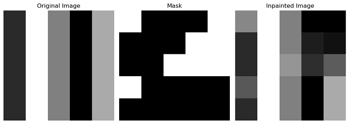
This example demonstrates the use of the inpaint_biharmonic() function to inpaint a damaged or missing region in an image based on a given mask.

import numpy as np
from skimage.restoration import inpaint_biharmonic
import matplotlib.pyplot as plt

# Create an example image
img = np.array([[ 1, 6,  3,  0,  4],
   [ 1, 6,  3,  0,  4],
   [ 1, 6,  3,  0,  4],
   [ 1, 6,  3,  0,  4],
   [ 1, 6,  3,  0,  4]], dtype='int32')

# Create a mask with known and unknown pixels
mask = np.zeros_like(img)
mask[2, 2:] = 1
mask[1, 3:] = 1
mask[0, 4:] = 1
mask[3, 0] = 1
mask[0, 0] = 1

# Perform inpainting using biharmonic equations
out = inpaint_biharmonic(img, mask)

# Visualize the original and inpainted images
fig, axes = plt.subplots(1, 3, figsize=(10, 5))

# Original Image
axes[0].imshow(img, cmap='gray')
axes[0].set_title('Original Image')
axes[0].axis('off')

# Mask
axes[1].imshow(mask, cmap='gray')
axes[1].set_title('Mask')
axes[1].axis('off')

# Inpainted Image
axes[2].imshow(out, cmap='gray')
axes[2].set_title('Inpainted Image')
axes[2].axis('off')

plt.tight_layout()
plt.show()

Output

Example

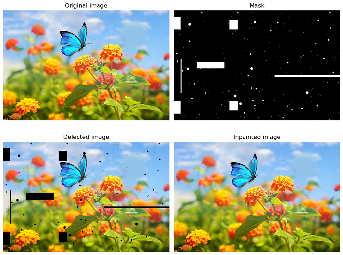
This example demonstrates how the inpaint_biharmonic() function is used to restore the defected regions in the image.

import numpy as np
import matplotlib.pyplot as plt
from skimage import io
from skimage.morphology import disk, binary_dilation
from skimage.restoration import inpaint

# Load the input image 
image = io.imread('Images/butterfly1.jpg')

# Create a mask with multiple defect regions
mask = np.zeros(image.shape[:-1], dtype=bool)

# Define and add six block defect regions
mask[20:60, 0:20] = 1
mask[160:180, 70:155] = 1
mask[30:60, 170:195] = 1
mask[-60:-30, 170:195] = 1
mask[-180:-160, 70:155] = 1
mask[-60:-20, 0:20] = 1

# Add a few long, narrow defects
mask[200:205, -200:] = 1
mask[150:255, 20:23] = 1
mask[365:368, 60:130] = 1

# Add randomly positioned small point-like defects
rstate = np.random.default_rng(0)
for radius in [0, 2, 4]:
   # Larger defects are less common
   # Make larger defects less common
   thresh = 3 + 0.25 * radius  
   tmp_mask = rstate.standard_normal(image.shape[:-1]) > thresh
   if radius > 0:
      tmp_mask = binary_dilation(tmp_mask, disk(radius, dtype=bool))
   mask[tmp_mask] = 1

# Apply the defect mask to the original image to create a defected image
image_defect = image * ~mask[..., np.newaxis]

# Use inpainting to restore the defected regions in the image
image_result = inpaint.inpaint_biharmonic(image_defect, mask, channel_axis=-1)

# Create subplots for visualization
fig, axes = plt.subplots(ncols=2, nrows=2, figsize=(10,8))
ax = axes.ravel()

ax[0].set_title('Original image')
ax[0].imshow(image)

ax[1].set_title('Mask')
ax[1].imshow(mask, cmap=plt.cm.gray)

ax[2].set_title('Defected image')
ax[2].imshow(image_defect)

ax[3].set_title('Inpainted image')
ax[3].imshow(image_result)

for a in ax:
   a.axis('off')
    
fig.tight_layout()
plt.show()

Output