Scikit Image - Masked Normalized Cross-Correlation

Masked Normalized Cross-Correlation is an image registration method designed to align images while accommodating the presence of masks or regions of interest within those images. It operates in the Fourier domain using normalized cross-correlation and efficiently incorporates masking to selectively consider or ignore regions of an image during registration. It is well-suited for fast and accurate registration in various computer vision and image analysis applications.

In this tutorial, we use the masked normalized cross-correlation method to determine the relative shift between two similar images containing areas with corrupted or invalid data.

In this context, it's not feasible to apply the masks to the images before computing the cross-correlation, as this would influence the computation. To address this, we need to eliminate the influence of the masks from the cross-correlation results.

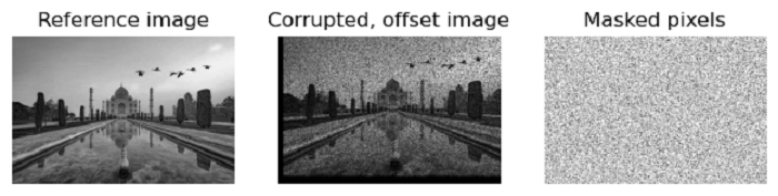
Example

In this example, our goal is to register the translation between two images. However, one of these images has approximately 25% of its pixels corrupted.

import numpy as np
import matplotlib.pyplot as plt

from skimage import io
from skimage.registration import phase_cross_correlation
from scipy import ndimage as ndi

# Load an image
image = io.imread('Images/Blue.jpg')

# Define a known shift in pixels
shift = (-22, 13)

# Add the random invalid data
rng = np.random.default_rng()
corrupted_pixels = rng.choice([False, True], size=image.shape, p=[0.25, 0.75])

# Apply the shift to create an offset image with corrupted pixels
offset_image = ndi.shift(image, shift)
offset_image *= corrupted_pixels
print(f'Known offset (row, col): {shift}')

# Create a mask based on the locations of the corrupted pixels
# In this case, the mask is known since we introduced the corruption
mask = corrupted_pixels

# Perform pixel precision image registration
detected_shift = phase_cross_correlation(image, offset_image, reference_mask=mask)

print(f'Detected pixel offset (row, col): {-detected_shift}')

# Create subplots to display results
fig, (ax1, ax2, ax3) = plt.subplots(1, 3, sharex=True, sharey=True, figsize=(8, 3))

ax1.imshow(image, cmap='gray')
ax1.set_axis_off()
ax1.set_title('Reference image')

ax2.imshow(offset_image.real, cmap='gray')
ax2.set_axis_off()
ax2.set_title('Corrupted, offset image')

ax3.imshow(mask, cmap='gray')
ax3.set_axis_off()
ax3.set_title('Masked pixels')

plt.show()

Output

Known offset (row, col): (-22, 13)
Detected pixel offset (row, col): [-22.  13.]

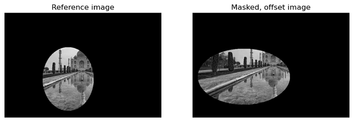
Using Solid masks

Solid masks provide another illustrative example. In this scenario, we have a limited view of both the reference image and an offset image. Notably, the masks applied to these images need not be the same. The phase_cross_correlation function effectively identifies, which part of the images should be compared.

Example

The following example demonstrates the use of the phase_cross_correlation function for pixel-precision image registration while considering solid masks.

import numpy as np
import matplotlib.pyplot as plt

from skimage import io, draw
from skimage.registration import phase_cross_correlation
from scipy import ndimage as ndi

# Load an image
image = io.imread('Images/Blue.jpg')

# Define a known shift in pixels
shift = (-22, 13)

# Create two solid masks using draw.ellipse
rr1, cc1 = draw.ellipse(259, 248, r_radius=125, c_radius=100, shape=image.shape)
rr2, cc2 = draw.ellipse(250, 200, r_radius=110, c_radius=180, shape=image.shape)

# Initialize mask arrays
mask1 = np.zeros_like(image, dtype=bool)
mask2 = np.zeros_like(image, dtype=bool)

# Set the corresponding pixels to True in the masks
mask1[rr1, cc1] = True
mask2[rr2, cc2] = True

# Apply the shift to create an offset image
offset_image = ndi.shift(image, shift)

# Apply masks to the images
image *= mask1
offset_image *= mask2

print(f'Known offset (row, col): {shift}')

# Perform pixel precision image registration with masking
detected_shift = phase_cross_correlation(image, offset_image,
   reference_mask=mask1,
   moving_mask=mask2)

print(f'Detected pixel offset (row, col): {-detected_shift}')

# Create subplots to display the reference image and the masked, offset image
fig = plt.figure(figsize=(10, 5))
ax1 = plt.subplot(1, 2, 1)
ax2 = plt.subplot(1, 2, 2, sharex=ax1, sharey=ax1)

ax1.imshow(image, cmap='gray')
ax1.set_axis_off()
ax1.set_title('Reference image')

ax2.imshow(offset_image.real, cmap='gray')
ax2.set_axis_off()
ax2.set_title('Masked, offset image')

plt.show()

Output

Known offset (row, col): (-22, 13)
Detected pixel offset (row, col): [-22.  13.]