Scikit Image - Wavelet Denoising

Wavelet denoising is a powerful technique for removing noise from images while preserving important image details. This technique is relies on the wavelet representation of an image. Gaussian noise in images is often characterized by small values in the wavelet domain. To remove this noise, wavelet denoising involves one of two main approaches −

• Hard Thresholding: This approach sets wavelet coefficients below a certain threshold to zero.

• Soft Thresholding: In soft thresholding, all wavelet coefficients are shrunk towards zero by a certain amount.

The scikit-image library provides a function within its restoration module that allows you to perform wavelet denoising on images. The function is called denoise_wavelet().

Using the skimage.restoration.denoise_wavelet() function

The restoration.denoise_wavelet() function is used to perform wavelet denoising on an image.

Syntax

Following is the syntax of this function −

skimage.restoration.denoise_wavelet(image, sigma=None, wavelet='db1', mode='soft', wavelet_levels=None, convert2ycbcr=False, method='BayesShrink', rescale_sigma=True, *, channel_axis=None)

Parameters

Below are the details of its parameters −

• image (ndarray): The input data (image) to be denoised. The image can be of any numeric type, but it is cast into an ndarray of floats for the denoising computation.

• sigma (float or list, optional): The noise standard deviation used when computing the wavelet detail coefficient threshold(s). When set to None (default), the noise standard deviation is estimated automatically via a method described in [D. L. Donoho and I. M. Johnstone. "Ideal spatial adaptation by wavelet shrinkage."

• wavelet (string, optional): The type of wavelet to use for denoising. It can be any of the wavelets available in PyWavelets (output of pywt.wavelist). The default is 'db1', but you can choose from options like 'db2', 'haar', 'sym9', and more.

• mode (string, optional): An argument to choose the type of denoising performed. It can be 'soft' or 'hard'. The choice of 'soft' thresholding is recommended for additive noise to find the best approximation of the original image.

• wavelet_levels (int or None, optional): The number of wavelet decomposition levels to use. The default is three less than the maximum number of possible decomposition levels.

• convert2ycbcr (bool, optional): If set to True and channel_axis is specified, the wavelet denoising is performed in the YCbCr colorspace instead of the RGB colorspace. This can improve performance for RGB images.

• method (string, optional): The thresholding method to be used. Supported methods are 'BayesShrink' (default) and 'VisuShrink'.

  • VisuShrink: it applies a single, universal threshold to all wavelet detail coefficients. This threshold is designed to remove additive Gaussian noise with a high probability. However, it can sometimes lead to an overly smooth appearance in the denoised image. To obtain more visually appealing results, you can specify a sigma (noise standard deviation) that is smaller than the true noise standard deviation.

  • BayesShrink: it is an adaptive approach to wavelet soft thresholding. It estimates a unique threshold for each wavelet subband. This adaptability generally results in better denoising compared to using a single threshold for the entire image.

• rescale_sigma (bool, optional): If False, no rescaling of the user-provided sigma will be performed. The default is True, which rescales Sigma appropriately if the image is rescaled internally. This parameter was introduced in version 0.16 of scikit-image.

• channel_axis (int or None, optional): If None, the image is assumed to be grayscale (single-channel). Otherwise, this parameter indicates which axis of the array corresponds to channels. This parameter was added in version 0.19 of scikit-image.

The function returns the denoised image as a ndarray.

Example

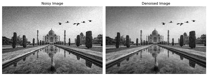
The following example demonstrates how to denoise an image using the wavelet-based denoising denoise_wavelet() function.

import numpy as np
import matplotlib.pyplot as plt
from skimage import color, io
from skimage import img_as_float
from skimage.restoration import denoise_wavelet

# Load the astronaut image and convert it to grayscale
img = img_as_float(io.imread('Images/Tajmahal_2.jpg'))
img = color.rgb2gray(img)

# Add Gaussian noise to the image
rng = np.random.default_rng()
img += 0.1 * rng.standard_normal(img.shape)

# Clip pixel values to the range [0, 1]
img = np.clip(img, 0, 1)

# Denoise the noisy image using wavelet denoising
denoised_img = denoise_wavelet(img, sigma=0.1, rescale_sigma=True)

# Visualize the original noisy image and the denoised image
fig, axes = plt.subplots(1, 2, figsize=(10, 10))
ax1, ax2 = axes.ravel()

ax1.imshow(img, cmap='gray')
ax1.set_title('Noisy Image')

ax2.imshow(denoised_img, cmap='gray')
ax2.set_title('Denoised Image')

for ax in axes:
   ax.axis('off')

plt.tight_layout()
plt.show()

Output

Example

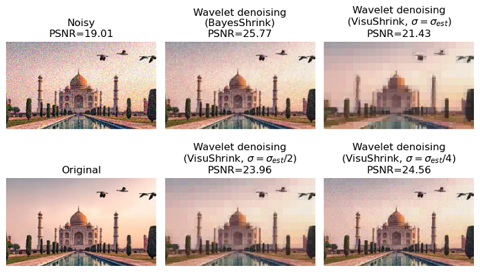
In the example, two different methods for selecting wavelet coefficient thresholds are illustrated: VisuShrink and BayesShrink.

import matplotlib.pyplot as plt
from skimage.restoration import (denoise_wavelet, estimate_sigma)
from skimage import io, img_as_float
from skimage.util import random_noise
from skimage.metrics import peak_signal_noise_ratio

# Load an example image 
original = img_as_float(io.imread('Images/Tajmahal.jpg'))

# Add Gaussian noise to the image
sigma = 0.12
noisy = random_noise(original, var=sigma**2)

# Estimate the average noise standard deviation across color channels
sigma_est = estimate_sigma(noisy, channel_axis=-1, average_sigmas=True)

# display the estimate of the Gaussian noise standard deviation
print(f'Estimated Gaussian noise standard deviation = {sigma_est}')

# Apply wavelet denoising with the BayesShrink method
im_bayes = denoise_wavelet(noisy, channel_axis=-1, convert2ycbcr=True,
   method='BayesShrink', mode='soft',
   rescale_sigma=True)

# Apply wavelet denoising with the VisuShrink method using estimated sigma
im_visushrink = denoise_wavelet(noisy, channel_axis=-1, convert2ycbcr=True,
   method='VisuShrink', mode='soft',
   sigma=sigma_est, rescale_sigma=True)

# Repeat VisuShrink with reduced threshold factors for visual comparison
im_visushrink2 = denoise_wavelet(noisy, channel_axis=-1, convert2ycbcr=True,
   method='VisuShrink', mode='soft',
   sigma=sigma_est/2, rescale_sigma=True)
im_visushrink4 = denoise_wavelet(noisy, channel_axis=-1, convert2ycbcr=True,
   method='VisuShrink', mode='soft',
   sigma=sigma_est/4, rescale_sigma=True)

# Compute PSNR (Peak Signal-to-Noise Ratio) as a measure of image quality
psnr_noisy = peak_signal_noise_ratio(original, noisy)
psnr_bayes = peak_signal_noise_ratio(original, im_bayes)
psnr_visushrink = peak_signal_noise_ratio(original, im_visushrink)
psnr_visushrink2 = peak_signal_noise_ratio(original, im_visushrink2)
psnr_visushrink4 = peak_signal_noise_ratio(original, im_visushrink4)

# Create a subplot for visualization
fig, axes = plt.subplots(nrows=2, ncols=3, figsize=(8, 5),
   sharex=True, sharey=True)
ax0, ax1, ax2, ax3, ax4, ax5 = axes.ravel()
plt.gray()

# Display the images and their PSNR values
ax0.imshow(noisy)
ax0.set_title(f'Noisy\nPSNR={psnr_noisy:0.4g}')
ax1.imshow(im_bayes)
ax1.set_title(
   f'Wavelet denoising\n(BayesShrink)\nPSNR={psnr_bayes:0.4g}')
ax2.imshow(im_visushrink)
ax2.set_title(
   'Wavelet denoising\n(VisuShrink, $\\sigma=\\sigma_{est}$)\n'
   'PSNR=%0.4g' % psnr_visushrink)
ax3.imshow(original)
ax3.set_title('Original')
ax4.imshow(im_visushrink2)
ax4.set_title(
   'Wavelet denoising\n(VisuShrink, $\\sigma=\\sigma_{est}/2$)\n'
   'PSNR=%0.4g' % psnr_visushrink2)
ax5.imshow(im_visushrink4)
ax5.set_title(
   'Wavelet denoising\n(VisuShrink, $\\sigma=\\sigma_{est}/4$)\n'
   'PSNR=%0.4g' % psnr_visushrink4)

for ax in axes.flat:
   ax.axis('off')

fig.tight_layout()
plt.show()

Output

Estimated Gaussian noise standard deviation = 0.10863181119379317