Scikit Image - Haar Like Feature Detection

Quiz

Haar-like feature detection is a technique used in digital image processing and object recognition. It is named after its resemblance to Haar wavelets. Paul Viola and Michael Jones adapted the idea of using Haar wavelets and developed the first real-time face detector using Haar-like features.

Haar-like features are used to identify objects or specific patterns within images. These features are characterized by their ability to consider adjacent rectangular regions at a particular location in a detection window and calculate the difference in pixel intensities between these regions. This difference is then used to classify and categorize subsections of an image.

The scikit-image library offers the haar_like_feature() function within its feature module to compute Haar-like features for a region of interest (ROI) within an integral image.

Using the skimage.feature.haar_like_feature() function

The skimage.feature.haar_like_feature function is used to compute Haar-like features for a region of interest (ROI) within an integral image. Haar-like features are often used in image classification and object detection tasks.

Syntax

Here is the syntax of this function −

skimage.feature.haar_like_feature(int_image, r, c, width, height, feature_type=None, feature_coord=None)

Parameters

The function has the following parameters −

int_image (M, N) ndarray: This is the integral image for which the Haar-like features need to be computed.
r (int): Row-coordinate of the top-left corner of the detection window (region of interest).
c (int): Column-coordinate of the top-left corner of the detection window (region of interest).
width (int): Width of the detection window (region of interest).
height (int): Height of the detection window (region of interest).
feature_type (str or list of str or None, optional): Specifies the type of Haar-like feature to consider. It can be one of the following −
- 'type-2-x': 2 rectangles varying along the x-axis.
- 'type-2-y': 2 rectangles varying along the y-axis.
- 'type-3-x': 3 rectangles varying along the x-axis.
- 'type-3-y': 3 rectangles varying along the y-axis.
- 'type-4': 4 rectangles varying along both x and y axes.
feature_coord (ndarray of list of tuples or None, optional): An array of coordinates to be extracted. This is useful when you want to recompute only a subset of features. If provided, feature_type should correspond to the feature type of each associated coordinate feature. By default, all coordinates are computed.

The function returns a NumPy array, haar_features, which is of shape (n_features,) and contains int or float values. Each value in this array is equal to the subtraction of sums of the positive and negative rectangles. The data type of haar_features depends on the data type of the int_image. It will be of type int when the data type of int_image is uint or int, and it will be of type float when the data type of int_image is float.

It's important to note that when extracting these features in parallel, the choice of the backend (i.e., multiprocessing vs. threading) can have an impact on performance. You should use multiprocessing when extracting features for all possible regions of interest (ROIs) in an image and use threading when extracting features at specific locations for a limited number of ROIs. The choice of backend depends on the specific use case and requirements for performance.

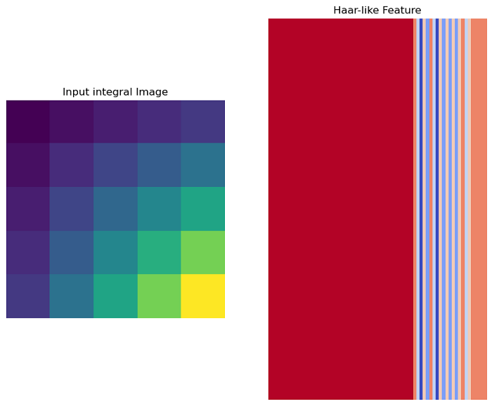
Example

This example computes the Haar-like feature of type 'type-3-x' for the entire 5x5 image using the skimage.feature.haar_like_feature() function.

import numpy as np
import matplotlib.pyplot as plt
from skimage.transform import integral_image
from skimage.feature import haar_like_feature

# Create a simple binary image (5x5) for illustration
img = np.ones((5, 5), dtype=np.uint8)

# Compute the integral image
img_ii = integral_image(img)

# Compute the Haar-like feature for the entire image
feature = haar_like_feature(img_ii, 0, 0, 5, 5, 'type-3-x')

# Display the original and the computed Haar-like feature
fig, axes = plt.subplots(1, 2, figsize=(10, 8))
ax = axes.ravel()

ax[0].imshow(img_ii)
ax[0].set_title('Input integral Image')
ax[0].axis('off')

# Display the computed Haar-like feature
ax[1].imshow(feature.reshape(1, -1), cmap='coolwarm', aspect='auto')
ax[1].set_title('Haar-like Feature')
ax[1].axis('off')
plt.show()

Output

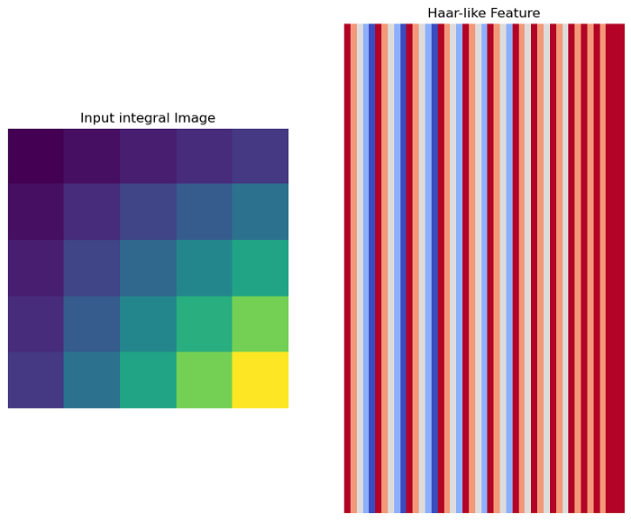
Additionally, the haar_like_feature() function can be used to compute the feature for some pre-computed coordinates.

Example

Here is the example, that uses the haar_like_feature_coord() and the haar_like_feature() functions to compute the Haar-lik feature for some pre-computed coordinates.

import numpy as np
import matplotlib.pyplot as plt
from skimage.transform import integral_image
from skimage.feature import haar_like_feature, haar_like_feature_coord

# Create a simple binary image (5x5) 
img = np.ones((5, 5), dtype=np.uint8)

# Compute the integral image
img_ii = integral_image(img)

# Define the feature coordinates and types
feature_coord, feature_type = zip(
   *[haar_like_feature_coord(5, 5, feat_t)
   for feat_t in ('type-2-x', 'type-3-x')])

# only select one feature over two
feature_coord = np.concatenate([x[::2] for x in feature_coord])
feature_type = np.concatenate([x[::2] for x in feature_type])

# Compute the Haar-like feature for the specified coordinates
feature = haar_like_feature(img_ii, 0, 0, 5, 5,
   feature_type=feature_type,
   feature_coord=feature_coord)

# Display the original and the computed Haar-like feature
fig, axes = plt.subplots(1, 2, figsize=(10, 8))
ax = axes.ravel()

ax[0].imshow(img_ii)
ax[0].set_title('Input integral Image')
ax[0].axis('off')

# Display the computed Haar-like feature
ax[1].imshow(feature.reshape(1, -1), cmap='coolwarm', aspect='auto')
ax[1].set_title('Haar-like Feature')
ax[1].axis('off')
plt.show()

# Print the computed Haar-like feature
print("Computed Haar-like Feature:", feature)

Output

Computed Haar-like Feature: 

[ 0  0  0  0  0  0  0  0  0  0  0  0  0  0  0  0  0  0  0  0  0  0  0  0
  0  0  0  0  0  0  0  0  0  0  0  0  0  0  0  0  0  0  0  0  0 -1 -3 -5
 -2 -4 -1 -3 -5 -2 -4 -2 -4 -2 -4 -2 -1 -3 -2 -1 -1 -1 -1 -1]

Print Page