- Scikit Image – Introduction
- Scikit Image - Image Processing
- Scikit Image - Numpy Images
- Scikit Image - Image datatypes
- Scikit Image - Using Plugins
- Scikit Image - Image Handlings
- Scikit Image - Reading Images
- Scikit Image - Writing Images
- Scikit Image - Displaying Images
- Scikit Image - Image Collections
- Scikit Image - Image Stack
- Scikit Image - Multi Image
- Scikit Image - Data Visualization
- Scikit Image - Using Matplotlib
- Scikit Image - Using Ploty
- Scikit Image - Using Mayavi
- Scikit Image - Using Napari
- Scikit Image - Color Manipulation
- Scikit Image - Alpha Channel
- Scikit Image - Conversion b/w Color & Gray Values
- Scikit Image - Conversion b/w RGB & HSV
- Scikit Image - Conversion to CIE-LAB Color Space
- Scikit Image - Conversion from CIE-LAB Color Space
- Scikit Image - Conversion to luv Color Space
- Scikit Image - Conversion from luv Color Space
- Scikit Image - Image Inversion
- Scikit Image - Painting Images with Labels
- Scikit Image - Contrast & Exposure
- Scikit Image - Contrast
- Scikit Image - Contrast enhancement
- Scikit Image - Exposure
- Scikit Image - Histogram Matching
- Scikit Image - Histogram Equalization
- Scikit Image - Local Histogram Equalization
- Scikit Image - Tinting gray-scale images
- Scikit Image - Image Transformation
- Scikit Image - Scaling an image
- Scikit Image - Rotating an Image
- Scikit Image - Warping an Image
- Scikit Image - Affine Transform
- Scikit Image - Piecewise Affine Transform
- Scikit Image - ProjectiveTransform
- Scikit Image - EuclideanTransform
- Scikit Image - Radon Transform
- Scikit Image - Line Hough Transform
- Scikit Image - Probabilistic Hough Transform
- Scikit Image - Circular Hough Transforms
- Scikit Image - Elliptical Hough Transforms
- Scikit Image - Polynomial Transform
- Scikit Image - Image Pyramids
- Scikit Image - Pyramid Gaussian Transform
- Scikit Image - Pyramid Laplacian Transform
- Scikit Image - Swirl Transform
- Scikit Image - Morphological Operations
- Scikit Image - Erosion
- Scikit Image - Dilation
- Scikit Image - Black & White Tophat Morphologies
- Scikit Image - Convex Hull
- Scikit Image - Generating footprints
- Scikit Image - Isotopic Dilation & Erosion
- Scikit Image - Isotopic Closing & Opening of an Image
- Scikit Image - Skelitonizing an Image
- Scikit Image - Morphological Thinning
- Scikit Image - Masking an image
- Scikit Image - Area Closing & Opening of an Image
- Scikit Image - Diameter Closing & Opening of an Image
- Scikit Image - Morphological reconstruction of an Image
- Scikit Image - Finding local Maxima
- Scikit Image - Finding local Minima
- Scikit Image - Removing Small Holes from an Image
- Scikit Image - Removing Small Objects from an Image
- Scikit Image - Filters
- Scikit Image - Image Filters
- Scikit Image - Median Filter
- Scikit Image - Mean Filters
- Scikit Image - Morphological gray-level Filters
- Scikit Image - Gabor Filter
- Scikit Image - Gaussian Filter
- Scikit Image - Butterworth Filter
- Scikit Image - Frangi Filter
- Scikit Image - Hessian Filter
- Scikit Image - Meijering Neuriteness Filter
- Scikit Image - Sato Filter
- Scikit Image - Sobel Filter
- Scikit Image - Farid Filter
- Scikit Image - Scharr Filter
- Scikit Image - Unsharp Mask Filter
- Scikit Image - Roberts Cross Operator
- Scikit Image - Lapalace Operator
- Scikit Image - Window Functions With Images
- Scikit Image - Thresholding
- Scikit Image - Applying Threshold
- Scikit Image - Otsu Thresholding
- Scikit Image - Local thresholding
- Scikit Image - Hysteresis Thresholding
- Scikit Image - Li thresholding
- Scikit Image - Multi-Otsu Thresholding
- Scikit Image - Niblack and Sauvola Thresholding
- Scikit Image - Restoring Images
- Scikit Image - Rolling-ball Algorithm
- Scikit Image - Denoising an Image
- Scikit Image - Wavelet Denoising
- Scikit Image - Non-local means denoising for preserving textures
- Scikit Image - Calibrating Denoisers Using J-Invariance
- Scikit Image - Total Variation Denoising
- Scikit Image - Shift-invariant wavelet denoising
- Scikit Image - Image Deconvolution
- Scikit Image - Richardson-Lucy Deconvolution
- Scikit Image - Recover the original from a wrapped phase image
- Scikit Image - Image Inpainting
- Scikit Image - Registering Images
- Scikit Image - Image Registration
- Scikit Image - Masked Normalized Cross-Correlation
- Scikit Image - Registration using optical flow
- Scikit Image - Assemble images with simple image stitching
- Scikit Image - Registration using Polar and Log-Polar
- Scikit Image - Feature Detection
- Scikit Image - Dense DAISY Feature Description
- Scikit Image - Histogram of Oriented Gradients
- Scikit Image - Template Matching
- Scikit Image - CENSURE Feature Detector
- Scikit Image - BRIEF Binary Descriptor
- Scikit Image - SIFT Feature Detector and Descriptor Extractor
- Scikit Image - GLCM Texture Features
- Scikit Image - Shape Index
- Scikit Image - Sliding Window Histogram
- Scikit Image - Finding Contour
- Scikit Image - Texture Classification Using Local Binary Pattern
- Scikit Image - Texture Classification Using Multi-Block Local Binary Pattern
- Scikit Image - Active Contour Model
- Scikit Image - Canny Edge Detection
- Scikit Image - Marching Cubes
- Scikit Image - Foerstner Corner Detection
- Scikit Image - Harris Corner Detection
- Scikit Image - Extracting FAST Corners
- Scikit Image - Shi-Tomasi Corner Detection
- Scikit Image - Haar Like Feature Detection
- Scikit Image - Haar Feature detection of coordinates
- Scikit Image - Hessian matrix
- Scikit Image - ORB feature Detection
- Scikit Image - Additional Concepts
- Scikit Image - Render text onto an image
- Scikit Image - Face detection using a cascade classifier
- Scikit Image - Face classification using Haar-like feature descriptor
- Scikit Image - Visual image comparison
- Scikit Image - Exploring Region Properties With Pandas
Scikit Image - Masking an Image
Masking an image is a fundamental technique in image processing and it's used for a wide range of tasks such as region of interest selection, image segmentation, and selective filtering. Applying a mask to an image, effectively "cover-ups" or "reveal" specified parts of the image based on the mask's regions. This allows you to perform various operations on the selected regions while leaving the rest of the image unaffected.
The scikit-image (skimage) library provides functions like flood() and flood_fill() that enable users to perform flood fill operations on images.
Using the skimage.morphology.flood() function
The morphology.flood() function is used for flood filling regions in an n-dimensional array. It starts from a specified seed point and fills connected points that are equal to or within a certain tolerance of the seed value found.
Syntax
Following is the syntax of this function −
skimage.morphology.flood(image, seed_point, *, footprint=None, connectivity=None, tolerance=None)
Parameters
- image (ndarray): An n-dimensional array on which flood fill will be performed.
- seed_point (tuple or int): The starting point for the flood fill. If the image is 1D, you can specify this point as an integer.
- footprint (ndarray, optional): This is the footprint (structuring element) used to determine the neighborhood of each evaluated pixel. It should contain only 1's and 0's and must have the same number of dimensions as the image. If not provided, all adjacent pixels are considered part of the neighborhood (fully connected).
- connectivity (int, optional): A number used to determine the neighborhood of each evaluated pixel. Pixels whose squared distance from the center is less than or equal to connectivity are considered neighbors. This parameter is ignored if footprint is not None.
- tolerance (float or int, optional): If set to None (default), adjacent values must be strictly equal to the initial value of the image at the seed_point. If a value is provided, a comparison will be done at every point, and if the value is within tolerance of the initial value, it will also be filled (inclusive).
Return Value
It returns a Boolean array with the same shape as the input image. It has True values for areas connected to and equal (or within tolerance of) the seed point and False for all other values.
Example
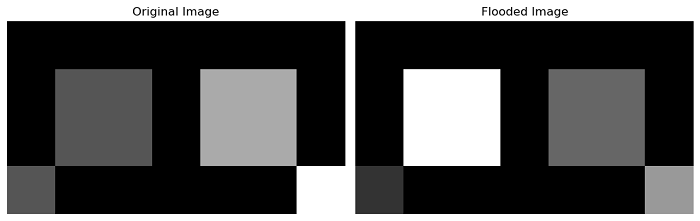
The following example demonstrates how to use the morphology.flood() function to perform a flood fill operation.
import numpy as np
from skimage.morphology import flood
import matplotlib.pyplot as plt

# Create an example image
image = np.zeros((4, 7), dtype=int)
image[1:3, 1:3] = 1
image[3, 0] = 1
image[1:3, 4:6] = 2
image[3, 6] = 3

# Perform flood fill starting from (1, 1)
mask = flood(image, (1, 1), connectivity=1)
image_flooded = image.copy()
image_flooded[mask] = 5

# Plot the original and thinned images
fig, axes = plt.subplots(1, 2, figsize=(10, 5))
ax = axes.ravel()

# Display the original binary image
ax[0].imshow(image, cmap=plt.cm.gray)
ax[0].axis('off')
ax[0].set_title('Original Image')

# Display the Thinned image
ax[1].imshow(image_flooded, cmap=plt.cm.gray)
ax[1].axis('off')
ax[1].set_title('Flooded Image')

plt.tight_layout()
plt.show()
Output
On executing the above program, you will get the following output −
Using the skimage.morphology.flood_fill() function
The morphology.flood_fill() function is used to perform flood filling on an image. It starts at a specified seed point and fills connected points that are equal to or within a certain tolerance of the seed value with a new specified value.
Syntax
Following is the syntax of this function −
skimage.morphology.flood_fill(image, seed_point, new_value, *, footprint=None, connectivity=None, tolerance=None, in_place=False)
Parameters
- image (ndarray): An n-dimensional array on which flood fill operation will be performed.
- seed_point (tuple or int): The starting point for the flood fill. If the image is 1D, you can specify this point as an integer.
- new_value (image type): The new value to set for the entire fill. This value must be chosen in agreement with the data type (dtype) of the image.
- footprint (ndarray, optional): The footprint (structuring element) used to determine the neighbourhood of each evaluated pixel. It should contain only 1's and 0's and must have the same number of dimensions as the image. If not provided, all adjacent pixels are considered part of the neighbourhood (fully connected).
- connectivity (int, optional): A number used to determine the neighbourhood of each evaluated pixel. Pixels whose squared distance from the centre is less than or equal to connectivity are considered neighbours. This parameter is ignored if the footprint is not None.
- tolerance (float or int, optional): If set to None (default), adjacent values must be strictly equal to the value of the image at the seed_point to be filled. If a tolerance is provided, adjacent points with values within plus or minus tolerance from the seed point are filled (inclusive).
- in_place (bool, optional): If True, flood filling is applied to the image in place. If False (default), the flood-filled result is returned without modifying the input image.
Return Value
It returns an array with the same shape as the input image, where values in areas connected to and equal (or within tolerance of) the seed point are replaced with new_value.
Example
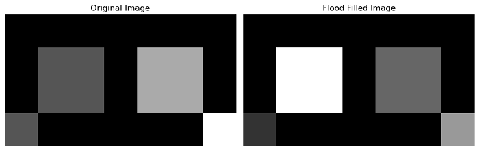
This example demonstrates how to use the morphology.flood_fill() function to perform a flood-fill operation on an image.
import numpy as np
from skimage.morphology import flood_fill
import matplotlib.pyplot as plt

# Create an example image
image = np.zeros((4, 7), dtype=int)
image[1:3, 1:3] = 1
image[3, 0] = 1
image[1:3, 4:6] = 2
image[3, 6] = 3

# Perform flood fill
filled_image = flood_fill(image, (1, 1), 5, connectivity=1)

# Plot the original and filled images
fig, axes = plt.subplots(1, 2, figsize=(10, 5))
ax = axes.ravel()

# Display the original binary image
ax[0].imshow(image, cmap=plt.cm.gray)
ax[0].axis('off')
ax[0].set_title('Original Image')

# Display the filled image
ax[1].imshow(filled_image, cmap=plt.cm.gray)
ax[1].axis('off')
ax[1].set_title('Flood Filled Image')

plt.tight_layout()
plt.show()
Output
On executing the above program, you will get the following output −