Face Classification using Haar-like Feature Descriptor

---

---

Haar-like feature descriptors are simple digital image features that are used in digital image processing and object recognition. These descriptors/features play a crucial role in identifying specific patterns or objects within images. They achieve this by analyzing the differences in pixel intensities between adjacent rectangular regions in a detection window, enabling the classification of image subsections.

In this tutorial, we demonstrate the process of extracting, selecting, and classifying Haar-like features to differentiate between faces and non-faces.

Please note that this example relies on scikit-learn for feature selection and classification.

The procedure for extracting Haar-like features from an image is relatively straightforward. First, a region of interest (ROI) is defined. Second, the integral image within this ROI is computed. Finally, the integral image is employed to extract the features.

We use a subset of the CBCL dataset, comprising 100 face images and 100 non-face images. Each image has been resized to an ROI of 19 by 19 pixels. We select 75 images from each group to train a classifier and identify the most important features. The remaining 25 images from each class are used to evaluate the classifier's performance.

To enhance computational efficiency without compromising accuracy, we can train a random forest classifier to identify the most important features, particularly for face classification. The concept is to determine which features are frequently used by the ensemble of trees. By using only the most prominent features in subsequent steps, we can significantly accelerate the computation while preserving accuracy.

Example

The following example demonstrates how to use Haar-like features and a random forest classifier for face classification.

from time import time
import numpy as np
import matplotlib.pyplot as plt
from sklearn.ensemble import RandomForestClassifier
from sklearn.model_selection import train_test_split
from sklearn.metrics import roc_auc_score
from skimage.data import lfw_subset
from skimage.transform import integral_image
from skimage.feature import haar_like_feature
from skimage.feature import haar_like_feature_coord
from skimage.feature import draw_haar_like_feature

def extract_haar_feature_image(img, feature_type, feature_coord=None):
   """Calculate Haar-like features for the given image"""
   integral_img = integral_image(img)
   return haar_like_feature(integral_img, 0, 0, integral_img.shape[0], integral_img.shape[1],
      feature_type=feature_type,
      feature_coord=feature_coord)

sample_images = lfw_subset()

# For efficiency, extract the two types of features only
selected_feature_types = ['type-2-x', 'type-2-y']

# Calculate the features
start_time = time()
X_features = [extract_haar_feature_image(img, selected_feature_types) for img in sample_images]
X_features = np.stack(X_features)
elapsed_time_feature_computation = time() - start_time

# Label the images (100 faces and 100 non-faces)
labels = np.array([1] * 100 + [0] * 100)

X_train, X_test, y_train, y_test = train_test_split(X_features, labels, train_size=150,
   random_state=0,
   stratify=labels)

# Extract all potential features
feature_coordinates, feature_types = haar_like_feature_coord(width=sample_images.shape[2], 
   height=sample_images.shape[1],
   feature_type=selected_feature_types)

# Train a random forest classifier and evaluate its performance
classifier = RandomForestClassifier(n_estimators=1000, max_depth=None,
   max_features=100, n_jobs=-1, random_state=0)
start_time = time()
classifier.fit(X_train, y_train)
elapsed_time_training = time() - start_time
auc_score_full_features = roc_auc_score(y_test, classifier.predict_proba(X_test)[:, 1])

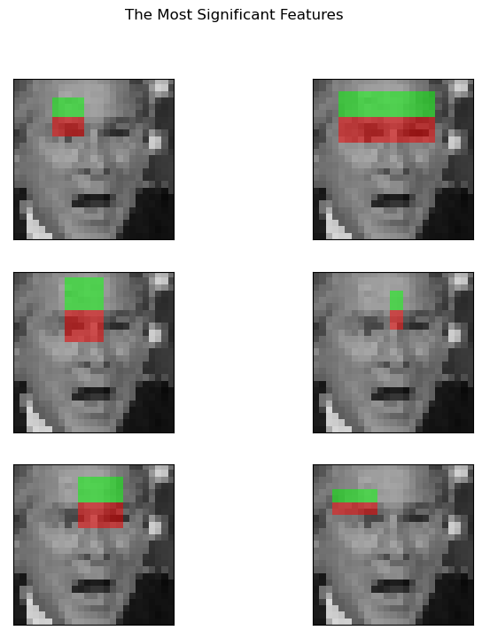
# Sort features by importance and display the top six
sorted_feature_indices = np.argsort(classifier.feature_importances_)[::-1]

fig, axes = plt.subplots(3, 2, figsize=(8, 8))
for idx, ax in enumerate(axes.ravel()):
   image = sample_images[0]
   image = draw_haar_like_feature(image, 0, 0,
      sample_images.shape[2],
      sample_images.shape[1],
      [feature_coordinates[sorted_feature_indices[idx]]])
   ax.imshow(image)
   ax.set_xticks([])
   ax.set_yticks([])

_ = fig.suptitle('The Most Significant Features')

Output

The selection of the most significant features is done by examining the cumulative sum of feature importance. In this example, we retain features that account for 70% of the cumulative value, which corresponds to using only 3% of the total number of features.

Example

Here is an example that demonstrates the process of feature selection based on the cumulative sum of the importance of features.

# Calculate the cumulative sum of feature importances and normalize
cdf_feature_importances = np.cumsum(classifier.feature_importances_[sorted_feature_indices])
cdf_feature_importances /= cdf_feature_importances[-1]  # Normalize by dividing by the maximum value

# Determine the number of significant features accounting for 70% of branch points
significant_feature_count = np.count_nonzero(cdf_feature_importances < 0.7)
significant_feature_percent = round(significant_feature_count / len(cdf_feature_importances) * 100, 1)

print('Significant_feature_count:')
print(f'{significant_feature_count} features, or {significant_feature_percent}%, '
      f'account for 70% of branch points in the random forest.')
print()

# Select the most informative features based on the determined count
selected_feature_coord = feature_coordinates[sorted_feature_indices[:significant_feature_count]]
selected_feature_type = feature_types[sorted_feature_indices[:significant_feature_count]]
# Note: You can also directly select features from the X matrix, but we're highlighting the use of `feature_coordinates` and `feature_types`
# to recompute a subset of desired features.

# Calculate the features using the selected subset
start_time = time()
X_selected = [
   extract_haar_feature_image(img, selected_feature_type, selected_feature_coord)
   for img in sample_images
]
X_selected = np.stack(X_selected)
elapsed_time_selected_feature_computation = time() - start_time

labels = np.array([1] * 100 + [0] * 100)
X_train, X_test, y_train, y_test = train_test_split(X_selected, labels, train_size=150,
   random_state=0,
   stratify=labels)

start_time = time()
classifier.fit(X_train, y_train)
elapsed_time_selected_training = time() - start_time

auc_selected_features = roc_auc_score(y_test, classifier.predict_proba(X_test)[:, 1])

result_summary = (
   f'Computing the full feature set took {elapsed_time_feature_computation:.3f}s, '
   f'plus {elapsed_time_training:.3f}s training, for an AUC of {auc_score_full_features:.2f}. '
   f'Computing the restricted feature set took {elapsed_time_selected_feature_computation:.3f}s, '
   f'plus {elapsed_time_selected_training:.3f}s training, for an AUC of {auc_selected_features:.2f}.'
)

print('Summary:')
print(result_summary)
plt.show()

Output

Significant_feature_count:
712 features, or 0.7%, account for 70% of branch points in the random forest.

Summary:
Computing the full feature set took 77.978s, plus 3.092s training, for an AUC of 1.00. Computing the restricted feature set took 0.159s, plus 2.488s training, for an AUC of 1.00.