Scikit Image - Image Registration

Quiz

Image registration is a fundamental process in image analysis and computer vision that refers to the process of overlaying two or more images acquired from different times, angles, or imaging sources to achieve geometric alignment for subsequent analysis.

In this tutorial, we use phase cross-correlation to identify the relative shift between two similar-sized images.

The scikit-image library provides the phase_cross_correlation function within its registration module to do this task. This function is uses cross-correlation in Fourier space, and optionally uses an upsampled matrix-multiplication DFT to achieve arbitrary subpixel precision.

Using the skimage.registration.phase_cross_correlation() function

The phase_cross_correlation() function is used for efficient subpixel image translation registration by cross-correlation.

This implementation offers the same precision comparable to that of FFT upsampled cross-correlation, while significantly reducing computation time and memory demands. It begins by estimating the initial cross-correlation peak using an FFT and subsequently enhances the accuracy of the shift estimation by the DFT upsampling only in a small neighborhood of that estimate, by means of a matrix-multiply DFT technique.

Syntax

Here is the syntax of the function −

skimage.registration.phase_cross_correlation(reference_image, moving_image, *, upsample_factor=1, space='real', disambiguate=False, return_error=True, reference_mask=None, moving_mask=None, overlap_ratio=0.3, normalization='phase')

Parameters

Following is the explanation of its parameters −

reference_image (array): The reference image.
moving_image (array): The image that you want to register with the reference image. It should have the same dimensionality as the reference image.
upsample_factor (int, optional): This parameter determines the factor for upsampling. It specifies how much the images will be registered to within 1 / upsample_factor of a pixel. For example, if upsample_factor is set to 20, the images will be registered within 1/20th of a pixel. The default is 1, meaning no upsampling.
space (string, optional): Defines how the algorithm interprets the input data. You can choose between "real" (the data will be FFT'd to compute the correlation) and "fourier" (data bypasses FFT of input data). This setting can affect the behavior of the algorithm, especially when masks are provided. It is case-insensitive.
disambiguate (bool): A boolean flag that controls whether the shift returned by the function is only accurate modulo the image shape due to the periodic nature of the Fourier transform. If set to True, it computes the real space cross-correlation for each possible shift, and the shift with the highest cross-correlation within the overlapping area is returned.
reference_mask (ndarray, optional): A boolean mask for the reference_image. This mask should evaluate to True (or 1) on valid pixels and has the same shape as the reference_image.
moving_mask (ndarray or None, optional): A boolean mask for the moving_image. If provided, it should evaluate to True (or 1) on valid pixels and have the same shape as the moving_image. If set to None, the reference_mask will be used.
overlap_ratio (float, optional): This parameter specifies the minimum allowed overlap ratio between the images. Translations with an overlap ratio lower than this threshold will be ignored. A lower overlap_ratio leads to a smaller maximum translation, while a higher overlap_ratio increases robustness against spurious matches caused by small overlap between masked images. This parameter is used when masks are provided.
normalization ({"phase", None}): The type of normalization to apply to the cross-correlation. If you specify "phase," it uses the "phase correlation" method. This parameter is unused when masks (reference_mask and moving_mask) are supplied.

The function returns the following −

shift (ndarray): The shift vector (in pixels) required to register the moving_image with the reference_image. The axis ordering is consistent with the axis order of the input array.
error (float): The translation-invariant normalized RMS error between the reference_image and moving_image. This value is not available when masks are used, in which case it returns NaN.
phasediff (float): The global phase difference between the two images, which should be zero if the images are non-negative. Like the error, this value is not available when masks are used, and it returns NaN.

Example

Here is an example that demonstrates the process of registering images and calculating the shift required to align them with pixel-level precision. The phase_cross_correlation() function is used to perform this pixel-precision image registration.

import numpy as np
import matplotlib.pyplot as plt

from skimage import io
from skimage.registration import phase_cross_correlation
from skimage.registration._phase_cross_correlation import _upsampled_dft
from scipy.ndimage import fourier_shift

# Load a sample image from the skimage library
image = io.imread('Images/Blue.jpg')

# Define a known shift in pixels
shift = (-22.4, 13.32)

# Apply the shift to create an offset image
offset_image = fourier_shift(np.fft.fftn(image), shift)
offset_image = np.fft.ifftn(offset_image)

# Print the known shift
print(f'Known offset (y, x): {shift}')

# Perform pixel precision image registration
shift, error, diffphase = phase_cross_correlation(image, offset_image)

# Create subplots to display the images and cross-correlation
fig = plt.figure(figsize=(10, 8))
ax1 = plt.subplot(1, 3, 1)
ax2 = plt.subplot(1, 3, 2, sharex=ax1, sharey=ax1)
ax3 = plt.subplot(1, 3, 3)

# Display the reference image
ax1.imshow(image, cmap='gray')
ax1.set_axis_off()
ax1.set_title('Reference image')

# Display the offset image
ax2.imshow(offset_image.real, cmap='gray')
ax2.set_axis_off()
ax2.set_title('Offset image')

# Show the cross-correlation result
image_product = np.fft.fft2(image) * np.fft.fft2(offset_image).conj()
cc_image = np.fft.fftshift(np.fft.ifft2(image_product))
ax3.imshow(cc_image.real)
ax3.set_axis_off()
ax3.set_title("Cross-correlation")

plt.show()

# Print the detected pixel offset
print(f'Detected pixel offset (y, x): {shift}')

Output

Known offset (y, x): (-22.4, 13.32)

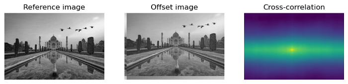
Detected pixel offset (y, x): [ 22. -13.]

Example

This example performs the subpixel precision image registration using the phase_cross_correlation function.

import numpy as np
import matplotlib.pyplot as plt

from skimage import io
from skimage.registration import phase_cross_correlation
from skimage.registration._phase_cross_correlation import _upsampled_dft
from scipy.ndimage import fourier_shift

# Load a sample image from the skimage library
image = io.imread('Images/Blue.jpg')

# Define a known shift in pixels
shift = (-22.4, 13.32)

# Apply the shift to create an offset image
offset_image = fourier_shift(np.fft.fftn(image), shift)
offset_image = np.fft.ifftn(offset_image)

# Perform subpixel precision image registration
shift, error, diffphase = phase_cross_correlation(image, offset_image, upsample_factor=100)

# Create subplots for subpixel registration
fig = plt.figure(figsize=(10, 8))
ax1 = plt.subplot(1, 3, 1)
ax2 = plt.subplot(1, 3, 2, sharex=ax1, sharey=ax1)
ax3 = plt.subplot(1, 3, 3)

# Display the reference image
ax1.imshow(image, cmap='gray')
ax1.set_axis_off()
ax1.set_title('Reference image')

# Display the offset image
ax2.imshow(offset_image.real, cmap='gray')
ax2.set_axis_off()
ax2.set_title('Offset image')

# Calculate the upsampled DFT for visualization
image_product = np.fft.fft2(image) * np.fft.fft2(offset_image).conj()
cc_image = _upsampled_dft(image_product, 150, 100, (shift * 100) + 75).conj()
ax3.imshow(cc_image.real)
ax3.set_axis_off()
ax3.set_title("Supersampled XC sub-area")

plt.show()

# Print the detected subpixel offset
print(f'Detected subpixel offset (y, x): {shift}')

Output

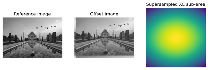
Detected subpixel offset (y, x): [ 22.4  -13.32]

Print Page