Scikit Image - GLCM Texture Features

Quiz

Gray-level co-occurrence matrices, often abbreviated as GLCMs, represent a fundamental concept in the field of image processing and computer vision. They serve as a powerful tool for analyzing and characterizing the complex textures present in digital images. Texture is a crucial visual attribute, plays a significant role in various applications, including object recognition, medical imaging, remote sensing, and more.

GLCMs is a histogram of co-occurring grayscale values at a given offset over an image.

The scikit image library has two functions, namely graycomatrix() and graycoprops() for calculating the gray-level co-occurrence matrix and extracting texture properties from a GLCM, respectively.

Using the skimage.feature.graycomatrix() function

The skimage.feature.graycomatrix() function is used for calculating the gray-level co-occurrence matrix (GLCM) from an input image.

Syntax

skimage.feature.graycomatrix(image, distances, angles, levels=None, symmetric=False, normed=False)

Parameters

Here are explanations of the parameters for the function −

image (array_like): It takes an input image, which should be of integer type. And it supports only positive-valued images. If the image type is not uint8, the argument levels needs to be set.
distances (array_like): A list of pixel pair distance offsets.
angles (array_like): A list of pixel pair angles in radians. It specifies the angles at which co-occurrence matrix will be computed.
levels (int, optional): This parameter requires 16-bit images or higher. It indicates the number of gray levels counted, typically 256 for an 8-bit image. The output matrix size is at least levels x levels. In some cases, it's preferable to use binning of the input image rather than large values for levels. The input image should contain integers in [0, levels-1], where levels indicate the number of gray-levels counted (typically 256 for an 8-bit image).
symmetric (bool, optional): If set to True, the output matrix P[:, :, d, theta] is made symmetric. This means it ignores the order of value pairs, so both (i, j) and (j, i) are accumulated when (i, j) is encountered for a given offset. The default value is False.
normed (bool, optional): When True, it normalizes each matrix P[:, :, d, theta] by dividing it by the total number of accumulated co-occurrences for the given offset. This ensures that the elements of the resulting matrix sum to 1. The default value is False.

The function returns a 4-Dimensional ndarray representing the gray-level co-occurrence histogram. The value P[i, j, d, theta] represents the number of times that gray-level j occurs at a distance d and at an angle theta from gray-level i. If normed is False, the output is of type uint32; otherwise, it is float64. The dimensions of the output matrix are levels x levels x number of distances x number of angles.

Example

Let's compute two Gray-Level Co-occurrence Matrices (GLCMs) for an input image. The first GLCM is calculated with a 1-pixel offset to the right, and the second GLCM is computed with a 1-pixel offset upwards.

import numpy as np
from skimage.feature import graycomatrix

# Define the input image
image = np.array([[0, 0, 1, 1],
   [0, 0, 1, 1],
   [0, 2, 2, 2],
   [2, 2, 3, 3]], dtype=np.uint8)

# Calculate the GLCM with specified parameters
result = graycomatrix(image, [1], [0, np.pi/4, np.pi/2, 3*np.pi/4], levels=4)

# Display the resulting GLCMs
print('Theta = 0')
print(result[:, :, 0, 0])
print('Theta = 1')
print(result[:, :, 0, 1])
print('Theta = 2')
print(result[:, :, 0, 2])
print('Theta = 3')
print(result[:, :, 0, 3])

Output

Theta = 0
[[2 2 1 0]
 [0 2 0 0]
 [0 0 3 1]
 [0 0 0 1]]

Theta = 1
[[1 1 3 0]
 [0 1 1 0]
 [0 0 0 2]
 [0 0 0 0]]

Theta = 2
[[3 0 2 0]
 [0 2 2 0]
 [0 0 1 2]
 [0 0 0 0]]

Theta = 3
[[2 0 0 0]
 [1 1 2 0]
 [0 0 2 1]
 [0 0 0 0]]

Using the skimage.feature.graycoprops() function

The skimage.feature.graycoprops() function is used to calculate various texture properties of a Gray-Level Co-occurrence Matrix (GLCM). Calculate a characteristic of a gray-level co-occurrence matrix to provide a compact summary of the matrix's properties. The properties are computed as follows −

contrast: $\mathrm{\sum_{i,j=0}^{levels-1} P_{i,j} (i-j)^2}$
dissimilarity: $\mathrm{\sum_{i,j=0}^{levels-1} P_{i,j} \lvert i-j\rvert}$
homogeneity: $\mathrm{\sum_{i,j=0}^{levels-1} \frac{P_{i,j}}{1+(i-j)^2}}$
ASM: $\mathrm{\sum_{i,j=0}^{levels-1} P_{i,j}^{2}}$
energy: $\mathrm{\sqrt{ASM}}$
correlation:$\mathrm{\sum_{i,j=0}^{levels-1}P_{i,j}\left[\frac{(i-\mu_{i})(j-\mu_{i})}{\sqrt{(\sigma_{i2})(\sigma_{j2})}} \right ]}$

Syntax

Here is the syntax of this method −

skimage.feature.graycoprops(P, prop='contrast')

Parameters

The method accepts the following parameters −

P (ndarray): This parameter takes the input array, which is the gray-level co-occurrence histogram (GLCM) for which to compute the specified property. The value P[i, j, d, theta] represents the number of times that gray-level j occurs at a distance d and at an angle theta from gray-level i.
prop (str, optional): It specifies the property of the GLCM to compute. It accepts the following options: 'contrast', 'dissimilarity', 'homogeneity', 'ASM', 'energy', 'correlation'. The default value is 'contrast'.

The function returns a 2-dimensional array where results[d, a] represents the property specified by prop for the d-th distance and the a-th angle.

Each GLCM is normalized to have a sum of 1 before the computation of these texture properties.

Example

The following example calculates the contrast properties from the gray-level co-occurrence matrix (GLCM) using the graycoprops() function.

import numpy as np
from skimage.feature import graycomatrix, graycoprops

# Define the input image
image = np.array([[0, 0, 1, 1],
   [0, 0, 1, 1],
   [0, 2, 2, 2],
   [2, 2, 3, 3]], dtype=np.uint8)

# Calculate the gray-level co-occurrence matrix (GLCM)
g = graycomatrix(image, [1, 2], [0, np.pi/2], levels=4,
   normed=True, symmetric=True)

# Compute the 'contrast' property from the GLCM
contrast = graycoprops(g, 'contrast')

# Print the 'contrast' property
print("Contrast:", contrast[0, 0])

Output

Contrast: 0.5833333333333333

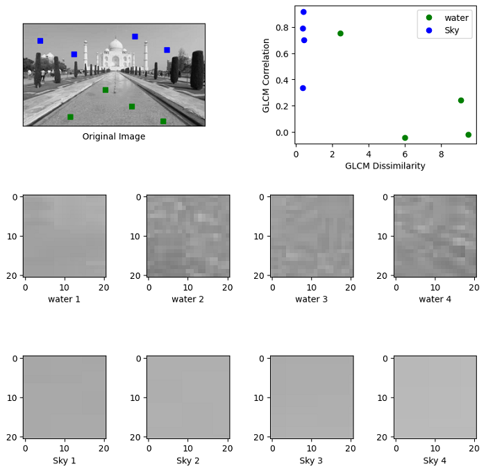
Example

This example demonstrates texture classification using the utilization of Gray Level Co-occurrence Matrices (GLCMs). Specifically, the example focuses on distinguishing between two distinct textures present in an image: water areas and sky areas.

For each selected patch within the image, a GLCM is computed with a horizontal offset of 5 (specified as distance=[5] and angles=[0]). Subsequently, two critical features, namely dissimilarity and correlation, are extracted from these GLCM matrices.

import matplotlib.pyplot as plt
from skimage.feature import graycomatrix, graycoprops
from skimage import io, util, exposure

PATCH_SIZE = 21

# open the input image
image = util.img_as_ubyte(io.imread('Images/Tajmahal_3.jpg', as_gray=True))
image = exposure.rescale_intensity(image)

# select some patches from water areas of the image
water_locations = [(160, 200), (230, 110), (202, 268), (240, 350)]
water_patches = []
for loc in water_locations:
   water_patches.append(image[loc[0]:loc[0] + PATCH_SIZE,
      loc[1]:loc[1] + PATCH_SIZE])

# select some patches from sky areas of the image
sky_locations = [(33, 33), (68, 119), (22, 276), (56, 359)]
sky_patches = []
for loc in sky_locations:
   sky_patches.append(image[loc[0]:loc[0] + PATCH_SIZE,
      loc[1]:loc[1] + PATCH_SIZE])

# compute some GLCM properties each patch
xs = []
ys = []
for patch in (water_patches + sky_patches):
   glcm = graycomatrix(patch, distances=[5], angles=[0], levels=256,
      symmetric=True, normed=True)
   xs.append(graycoprops(glcm, 'dissimilarity')[0, 0])
   ys.append(graycoprops(glcm, 'correlation')[0, 0])

# create the figure
fig = plt.figure(figsize=(8, 8))

# display original image with locations of patches
ax = fig.add_subplot(3, 2, 1)
ax.imshow(image, cmap=plt.cm.gray,
   vmin=0, vmax=255)
for (y, x) in water_locations:
   ax.plot(x + PATCH_SIZE / 2, y + PATCH_SIZE / 2, 'gs')
for (y, x) in sky_locations:
   ax.plot(x + PATCH_SIZE / 2, y + PATCH_SIZE / 2, 'bs')
ax.set_xlabel('Original Image')
ax.set_xticks([])
ax.set_yticks([])
ax.axis('image')

# for each patch, plot (dissimilarity, correlation)
ax = fig.add_subplot(3, 2, 2)
ax.plot(xs[:len(water_patches)], ys[:len(water_patches)], 'go',
   label='water')
ax.plot(xs[len(water_patches):], ys[len(water_patches):], 'bo',
   label='Sky')
ax.set_xlabel('GLCM Dissimilarity')
ax.set_ylabel('GLCM Correlation')
ax.legend()

# display the image patches
for i, patch in enumerate(water_patches):
   ax = fig.add_subplot(3, len(water_patches), len(water_patches)*1 + i + 1)
   ax.imshow(patch, cmap=plt.cm.gray,
      vmin=0, vmax=255)
   ax.set_xlabel(f"water {i + 1}")

for i, patch in enumerate(sky_patches):
   ax = fig.add_subplot(3, len(sky_patches), len(sky_patches)*2 + i + 1)
   ax.imshow(patch, cmap=plt.cm.gray,
      vmin=0, vmax=255)
   ax.set_xlabel(f"Sky {i + 1}")

plt.tight_layout()
plt.show()

Output

Print Page