Scikit Image - Contrast Enhancement

Quiz

Contrast enhancement is an image processing technique used to improve the visibility and quality of an image. It involves increasing the difference between the various elements within an image, such as objects, shapes, edges, and textures, by adjusting the distribution of intensity values or colors.

It can be useful when an image has poor contrast, meaning that the range between the darkest and lightest regions is limited, resulting in a flat and less informative appearance.

This technique is widely used in fields such as medical imaging, computer vision, remote sensing, and photography to improve image quality and get better visual information.

Pythons scikit-image library provides the rank.enhance_contrast() and rank.enhance_contrast_percentile() methods in the filters module to apply the contrast enhancing technique to an image.

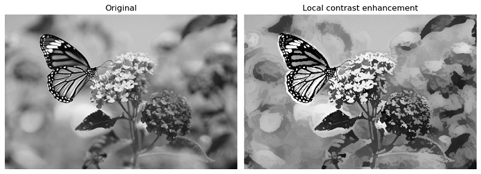
Using the skimage.filters.rank.enhance_contrast() method

The rank.enhance_contrast() function is used to enhance the contrast of an image by replacing each pixel with either the local maximum or the local minimum value, depending on which one is closer to the pixel's gray value within a local maximum or local minimum.

Syntax

Following is the syntax of this method −

skimage.filters.rank.enhance_contrast(image, footprint, out=None, mask=None, shift_x=False, shift_y=False, shift_z=False)

Parameters

image: This parameter represents the input image that you want to enhance contrast for.
footprint: It defines the local neighborhood where the operation is applied. It is represented as a binary ndarray of 1's and 0's.
out: If set to None, a new array is allocated for the result. The output array has the same data type as the input image.
mask (optional): This is an ndarray that can be used to mask the area of the image included in the local neighborhood. Pixels with values greater than 0 in the mask are included and the rest are excluded. If not specified (default is None), the entire image is used.
shift_x, shift_y, shift_z: These parameters specify the offset added to the center point of the footprint. The shift is bounded to the footprint sizes, meaning that the center must be inside the given footprint.

Return Value

It returns an output ndarray of the same shape and data type as the input image, containing the enhanced contrast image.

Example

The following example demonstrates how to enhance the contrast of a grayscale image using the enhance_contrast() function.

from skimage import io
from skimage.morphology import disk
from skimage.filters.rank import enhance_contrast
from skimage import img_as_ubyte
import matplotlib.pyplot as plt

# Load an example grayscale image
image = io.imread('Images/butterfly.jpg', as_gray=True)

noisy_image = img_as_ubyte(image)

# Apply the enhance_contrast() function to the image
penh = enhance_contrast(noisy_image, disk(5))

# Display the original and enhanced images side by side
fig, axes = plt.subplots(1, 2, figsize=(10, 10))
ax = axes.ravel()
ax[0].imshow(noisy_image, cmap=plt.cm.gray)
ax[0].set_title('Original')
ax[0].set_axis_off()

ax[1].imshow(penh, cmap=plt.cm.gray)
ax[1].set_title('Local contrast enhancement')
ax[1].set_axis_off()
plt.tight_layout()

plt.show()

Output

On executing the above program, you will get the following output −

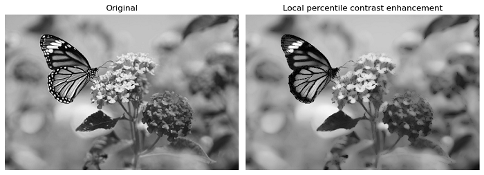
Using the skimage.filters.rank.enhance_contrast_percentile() method

The rank.enhance_contrast_percentile() method is used to enhance the contrast of an image by replacing each pixel with either the local maximum or the local minimum value, depending on whether the pixel's gray value falls within a specified percentile interval [p0, p1].