Scikit Image - Area Closing and Opening an Image

Quiz

Area closing and area opening are the image processing operations used to manipulate binary or grayscale images based on the size or surface area of objects in the image. Area closing is to remove all dark structures in an image (regions with lower intensity) that have a surface area smaller than a specified threshold, whereas area opening is to remove all bright structures in an image (regions with higher intensity) that have a surface area smaller than a specified threshold.

These operations are particularly useful for tasks such as removing small structures or objects from an image while preserving larger ones.

Scikit-image (skimage) provides the area_closing() and area_opening() functions in the morphology module to perform these operations.

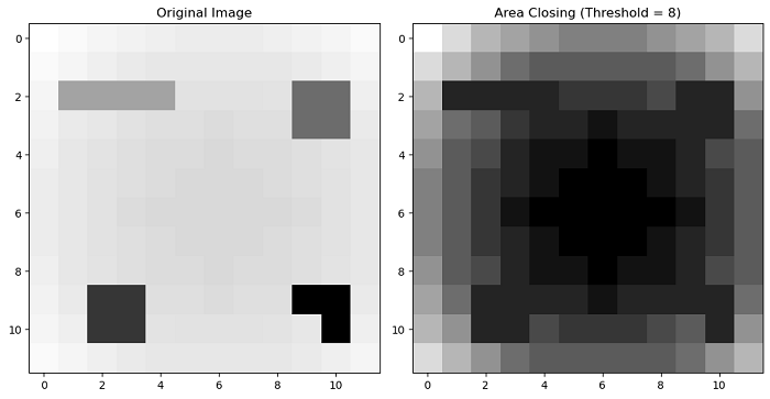
Using the skimage.morphology.area_closing() function

The area_closing() function is used to perform an area closing operation on an input image. Area closing removes dark structures in an image that have a surface (area) smaller than a specified threshold. This operation is similar to morphological closing, but instead of using a fixed structuring element, it employs a deformable one with a surface equal to the area_threshold.

Syntax

Following is the syntax of this function −

skimage.morphology.area_closing(image, area_threshold=64, connectivity=1, parent=None, tree_traverser=None)

Parameters

image (ndarray): The input image for which the area closing operation is to be performed. This image can be of any type.
area_threshold (unsigned int): The size parameter, specified in the number of pixels. It defines the minimum surface area that a dark structure must have to be retained. The default value is 64.
connectivity (unsigned int, optional): The neighborhood connectivity. This parameter specifies the maximum number of orthogonal steps to reach a neighbor. In 2D, it is typically set to 1 for a 4-neighborhood and 2 for an 8-neighborhood. The default value is 1.
parent (ndarray, int64, optional): A precomputed parent image representing the max tree of the inverted image. Providing a precomputed parent image can speed up the function. This parameter is optional.
tree_traverser (1D array, int64, optional): A precomputed traverser where the pixels are ordered such that every pixel is preceded by its parent (except for the root, which has no parent). Providing a precomputed traverser can also speed up the function. This parameter is optional.

Return Value

It returns an output image of the same shape and type as the input image, where dark structures with an area smaller than the specified threshold have been removed.

Example

The following example demonstrates how to apply the area_closing() function on an image.

import numpy as np
import matplotlib.pyplot as plt
from skimage.morphology import area_closing

# Create the image
w = 12
x, y = np.mgrid[0:w, 0:w]
image = 180 + 0.2 * ((x - w/2)**2 + (y - w/2)**2)

# Add local minima
image[2:3, 1:5] = 160
image[2:4, 9:11] = 140
image[9:11, 2:4] = 120
image[9:10, 9:11] = 100
image[10, 10] = 100

# Convert the image to integer
image = image.astype(int)

# Perform area closing with a threshold of 8 and connectivity=1
closed = area_closing(image, 8, connectivity=1)

# Display the original and closed images
fig, axes = plt.subplots(1, 2, figsize=(10, 5))
ax = axes.ravel()

ax[0].imshow(image, cmap=plt.cm.gray)
ax[0].set_title('Original Image')

ax[1].imshow(closed, cmap=plt.cm.gray)
ax[1].set_title('Area Closing (Threshold = 8)')
plt.tight_layout()
plt.show()

Output

On executing the above program, you will get the following output −

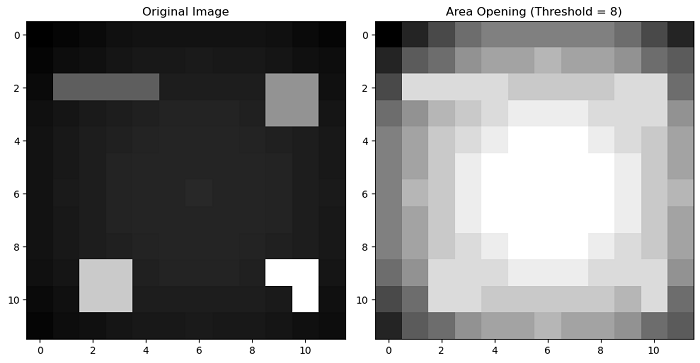
Using the skimage.morphology.area_opening() function

The area_opening() function is used to perform an area opening operation on an input image. Area opening removes bright structures in an image that have a surface area smaller than a specified threshold. This operation is similar to the morphological opening, but instead of using a fixed structuring element, it employs a deformable one with a surface area equal to the area_threshold.