Exploring Region Properties With Pandas

Exploring region properties with pandas, refers to the process of using the pandas library to analyze and manipulate region-related data. In the context of image processing region properties refer to characteristics or measurements associated with specific areas within an image, 2D or 3D, such as blobs or objects.

This tutorial provides two examples below that demonstrates the process of determining the size of labeled regions within a series of 10 images. We begin with 2D images and then transition to 3D images. These blob-like regions are synthetically generated. As the volume fraction, representing the proportion of pixels or voxels occupied by the blobs, increases, the number of these blobs (regions) decreases, leading to the potential for individual regions to get larger in size. The area (or volume) measurements are stored in a format compatible with pandas, facilitating easy data analysis and visualization.

In addition to the area, many other region properties are also available for further analysis.

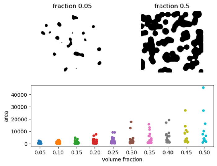
2D images

The following example demonstrates the process of generating synthetic 2D binary blob images, calculating region properties, and storing them in a pandas DataFrame. It is then used to visualize the relationship between the volume fraction and the size of regions through a scatter plot.

Example

import matplotlib.pyplot as plt
import numpy as np
import pandas as pd
import seaborn as sns

from skimage import data, measure

# Define the range of fractions
fractions = np.linspace(0.05, 0.5, 10)

# Generate binary blob images with different volume fractions
images = [data.binary_blobs(volume_fraction=f) for f in fractions]

# Label the generated binary images
labeled_images = [measure.label(image) for image in images]

# Define the properties of interest
properties = ['label', 'area']

# Measure region properties for each labeled image
tables = [measure.regionprops_table(image, properties=properties)
   for image in labeled_images]

# Convert the tables to DataFrames
tables = [pd.DataFrame(table) for table in tables]

# Add 'volume fraction' column to each DataFrame
for fraction, table in zip(fractions, tables):
   table['volume fraction'] = fraction

# Concatenate the DataFrames into a single DataFrame
areas = pd.concat(tables, axis=0)

# Create a custom grid of subplots
grid = plt.GridSpec(2, 2)
ax1 = plt.subplot(grid[0, 0])
ax2 = plt.subplot(grid[0, 1])
ax = plt.subplot(grid[1, :])

# Show the image with the lowest volume fraction
ax1.imshow(images[0], cmap='gray_r')
ax1.set_axis_off()
ax1.set_title(f'fraction {fractions[0]}')

# Show the image with the highest volume fraction
ax2.imshow(images[-1], cmap='gray_r')
ax2.set_axis_off()
ax2.set_title(f'fraction {fractions[-1]}')

# Plot area vs volume fraction
sns.stripplot(x='volume fraction', y='area', data=areas, jitter=True,
   ax=ax)

# Fix floating point rendering
ax.set_xticklabels([f'{frac:.2f}' for frac in fractions])
plt.show() 

Output

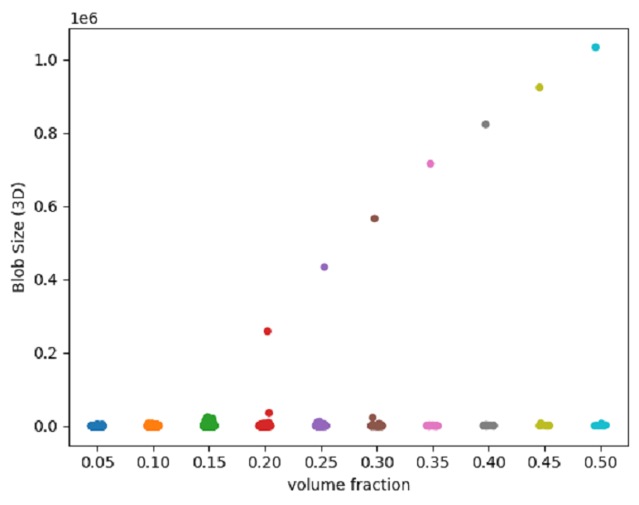
3D images

when performing the same analysis, a significantly more pronounced behavior is observed. As the volume fraction surpasses approximately 0.25, the blobs merge into a single massive entity. This corresponds to the percolation threshold observed in the fields of statistical physics and graph theory.

Example

Here is the example of exploring the region properties of 3D binary blob images using Pandas.

import matplotlib.pyplot as plt
import numpy as np
import pandas as pd
import seaborn as sns
from skimage import data, measure

# Define the range of volume fractions
fractions = np.linspace(0.05, 0.5, 10)

# Generate 3D binary blob images with specified volume fractions
images = [data.binary_blobs(length=128, n_dim=3, volume_fraction=f) for f in fractions]

# Label the 3D binary images
labeled_images = [measure.label(image) for image in images]

# Define the properties of interest
properties = ['label', 'area']

# Compute region properties for labeled 3D images
tables = [measure.regionprops_table(image, properties=properties) for image in labeled_images]

# Convert the result into Pandas DataFrames
tables = [pd.DataFrame(table) for table in tables]

# Assign volume fractions to each DataFrame
for fraction, table in zip(fractions, tables):
   table['volume fraction'] = fraction

# Concatenate all DataFrames into one
blob_volumes = pd.concat(tables, axis=0)

# Create a plot
fig, ax = plt.subplots()
sns.stripplot(x='volume fraction', y='area', data=blob_volumes, jitter=True, ax=ax)
ax.set_ylabel('Blob Size (3D)')

# Ensure proper rendering of x-axis labels
ax.set_xticklabels([f'{frac:.2f}' for frac in fractions])
plt.show()

Output