Scikit Image - Richardson-Lucy Deconvolution

The RichardsonLucy algorithm, also known as LucyRichardson deconvolution, is an iterative image processing technique used to recover an underlying image that has been degraded or blurred by a known point spread function (PSF). This technique was named after its independent discoverers, William Richardson and Leon B. Lucy.

The algorithm works based on a PSF (Point Spread Function), representing the impulse response of an optical system. Through multiple iterations, the blurred image is progressively sharpened, and it requires manual tuning for optimal results.

Scikit-image provides a dedicated function within its restoration module to perform Richardson-Lucy deconvolution on images.

Using the skimage.restoration.richardson_lucy() function

The restoration.richardson_lucy()function performs Richardson-Lucy deconvolution on an input degraded image.

Syntax

Here is the syntax of this function −

skimage.restoration.richardson_lucy(image, psf, num_iter=50, clip=True, filter_epsilon=None)

Parameters

The function accepts the following parameters −

• image(ndarray): Input degraded image, which can be n-dimensional.

• psf(ndarray): The point spread function.

• Num_iter (int, optional): Number of iterations for the Richardson-Lucy deconvolution algorithm. This parameter plays a role in controlling the regularization of the deconvolution process.

• clip (boolean, optional): If set to True (default), the pixel values of the result that are above 1 or below -1 are thresholded. This is done for compatibility with the scikit-image pipeline.

• filter_epsilon (float, optional): A value below which intermediate results become 0 to avoid division by small numbers. It helps stabilize the deconvolution process.

The function returns a ndarray(im_deconv), which represents the deconvolved image.

Example

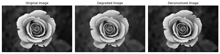
Here is an example that demonstrates the restoration of a noisy image (Gaussian noise) using the Richardson-Lucy algorithm.

import matplotlib.pyplot as plt
import numpy as np
from scipy.signal import convolve2d
from skimage import util, io, restoration

# Load the input image and convert it to a floating-point representation
image = util.img_as_float(io.imread('Images/black rose.jpg', as_gray=True))

# Define a point spread function (PSF) 
psf = np.ones((5, 5)) / 25

# Convolve (blur) the input image with the defined PSF
image_noisy = convolve2d(image, psf, 'same')

# Add noise to the original image
rng = np.random.default_rng()
image_noisy = image.copy()
image_noisy += 0.1 * image.std() * rng.standard_normal(image.shape)

# Apply Richardson-Lucy deconvolution for 5 iterations
deconvolved = restoration.richardson_lucy(image_noisy, psf, num_iter=5)

# Display the original image, degraded image, and deconvolved image side by side
fig, axes = plt.subplots(1, 3, figsize=(12, 4))

# Original Image
axes[0].imshow(image, cmap='gray')
axes[0].set_title('Original Image')
axes[0].axis('off')

# Degraded Image
axes[1].imshow(image_noisy, cmap='gray')
axes[1].set_title('Degraded Image')
axes[1].axis('off')

# Deconvolved Image
axes[2].imshow(deconvolved, cmap='gray')
axes[2].set_title('Deconvolved Image')
axes[2].axis('off')

plt.tight_layout()
plt.show()

Output

Example

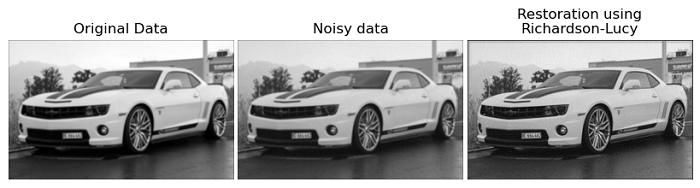
The following example demonstrates the restoration of a noisy image (Poisson noise) using the Richardson-Lucy algorithm.

import numpy as np
import matplotlib.pyplot as plt
from scipy.signal import convolve2d as conv2
from skimage import color, io, restoration

# Initialize a random number generator
rng = np.random.default_rng()

# Load the input image and convert it to grayscale
image = color.rgb2gray(io.imread('Images/Car_2.jpg'))

# Define a point spread function (PSF) 
psf = np.ones((5, 5)) / 25

# Convolve the input image with the PSF to simulate a blurred image
image = conv2(image, psf, 'same')

# Add Poisson noise to the blurred image
noisy_image = image.copy()
noisy_image += (rng.poisson(lam=25, size=image.shape) - 10) / 255.

# Restore the noisy image using the Richardson-Lucy algorithm
deconvolved_RL = restoration.richardson_lucy(noisy_image, psf, num_iter=30)

# Create subplots to display the original image, noisy image, and restored image
fig, ax = plt.subplots(1, 3, figsize=(8, 5))
plt.gray()

# Display the original image
ax[0].imshow(image)
ax[0].set_title('Original Data')

# Display the noisy image
ax[1].imshow(noisy_image)
ax[1].set_title('Noisy data')

# Display the restored image
ax[2].imshow(deconvolved_RL, vmin=noisy_image.min(), vmax=noisy_image.max())
ax[2].set_title('Restoration using\nRichardson-Lucy')

for a in (ax[0], ax[1], ax[2]):
   a.axis('off')

fig.subplots_adjust(wspace=0.02, hspace=0.2, top=0.9, bottom=0.05, left=0, right=1)
plt.show()

Output