Scikit Image - Image Deconvolution

Quiz

Image deconvolution is a computational technique used in image processing to recover or enhance the original image from a degraded or blurred version of that image.

In this tutorial, two different deconvolution algorithms (Wiener and unsupervised Wiener) are applied to a noisy image to enhance it. These algorithms are based on linear models and are known for their speed, although they may not restore sharp edges as effectively as non-linear methods like TV restoration.

The scikit-image (skimage) library provides functions for both Wiener and unsupervised Wiener deconvolution within its restoration module, namely 'wiener()' and 'unsupervised_wiener()'.

Using the Wiener-Hunt Deconvolution algorithm

The skimage.restoration.wiener() function is used for deconvolution with a Wiener-Hunt approach, which involves Fourier diagonalization. This function is used to enhance the quality of degraded images.

Syntax

Following is the syntax of this function −

skimage.restoration.wiener(image, psf, balance, reg=None, is_real=True, clip=True)

Parameters

The function accepts the following parameters −

image (ndarray): This parameter represents the input degraded image. It can be n-dimensional.
psf (ndarray): Point Spread Function (PSF) representing the impulse response in the image space if the data-type is real or the transfer function in Fourier space if the data-type is complex. There are no constraints on the shape of the impulse response. The transfer function must have a shape of (N1, N2, , ND) if is_real is True, or (N1, N2, , ND // 2 + 1).
balance (float): The balance parameter is a regularisation parameter that controls the balance between improving frequency restoration (data adequacy) and reducing noise artifacts (prior adequacy). It helps in controlling the deconvolution process.
reg (ndarray, optional): This is the regularisation operator, which is optional. By default, it uses the Laplacian. Like the PSF, the shape of the reg parameter depends on whether is_real is True or False. It can be provided in the impulse response or the transfer function.
is_real (boolean, optional): This parameter is True by default. It specifies whether psf and reg are provided with a hermitian hypothesis, which means they contain only half of the frequency plane due to the redundancy of the Fourier transform of real signals.
clip (boolean, optional): This parameter is True by default. If True, it clips pixel values in the result above 1 or below -1 are thresholded for skimage pipeline compatibility.

The function returns the deconvolved image, which is typically of shape (M, N). It represents the enhanced image after the Wiener-Hunt deconvolution.

Example

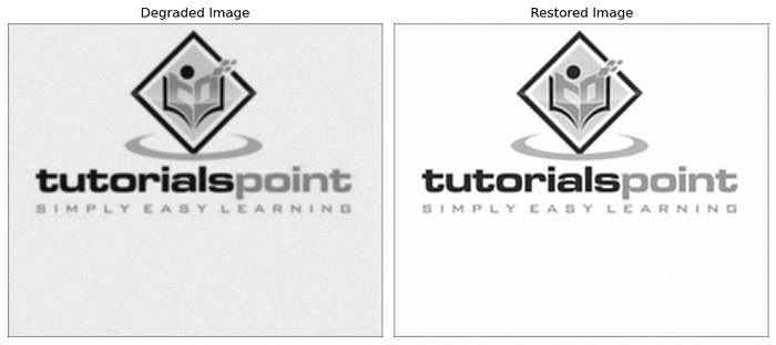
The following example demonstrates the use of the Wiener deconvolution technique to restore a degraded image.

import numpy as np
import matplotlib.pyplot as plt
from skimage import color, io, restoration
from scipy.signal import convolve2d

# Load the input image and convert it to grayscale
img = color.rgb2gray(io.imread('Images/logo.jpg'))

# Define a simple PSF (point spread function)
psf = np.ones((5, 5)) / 25

# Simulate image degradation by convolving with the PSF
img = convolve2d(img, psf, 'same')

# Add noise to the degraded image
rng = np.random.default_rng()
img += 0.1 * img.std() * rng.standard_normal(img.shape)

# Apply Wiener deconvolution to restore the image
deconvolved_img = restoration.wiener(img, psf, 0.1)

# Create subplots for visualization
fig, axes = plt.subplots(1, 2, figsize=(10, 10))
ax1, ax2 = axes.ravel()

# Original Image
ax1.imshow(img, cmap='gray')
ax1.set_title('Degraded Image')
ax1.axis('off')

# Degraded Image with Noise
ax2.imshow(deconvolved_img, cmap='gray')
ax2.set_title('Restored Image')
ax2.axis('off')

plt.tight_layout()
plt.show()

Output

Using the unsupervised Wiener algorithm

The restoration.unsupervised_wiener() function is used for unsupervised Wiener-Hunt deconvolution, which is a deconvolution technique where the hyperparameters are automatically estimated. This algorithm uses a stochastic iterative process (Gibbs sampler) for estimation.

Syntax

Following is the syntax of this function −

skimage.restoration.unsupervised_wiener(image, psf, reg=None, user_params=None, is_real=True, clip=True, *, rng=None)

Parameters

Here are the details of its parameters −

image (M, N) ndarray: The input degraded image on which deconvolution will be performed.
psf ndarray: The impulse response in the input image's space or the transfer function in Fourier space. Both types are accepted, and the transfer function is automatically recognized as complex.
reg ndarray, optional: The regularization operator, which defaults to the Laplacian. It can be an impulse response or a transfer function, similar to the psf parameter.
clip boolean, optional: True by default. If true, pixel values of the result above 1 or below -1 are thresholded for compatibility with the skimage pipeline.
rng {numpy.random.Generator, int}, optional: Pseudo-random number generator. By default, a PCG64 generator is used. If rng is an integer, it is used to seed the generator. (New in version 0.19)
user_params dict, optional: A dictionary of parameters for the Gibbs sampler. It includes the following keys −
- threshold (float): The stopping criterion, which is the norm of the difference between successive approximated solutions (empirical mean of object samples). Defaults to 1e-4.
- burnin (int): The number of samples to ignore at the start of the computation of the mean. Defaults to 15.
- min_num_iter (int): The minimum number of iterations. Defaults to 30.
- max_num_iter (int): The maximum number of iterations if the threshold is not satisfied. Defaults to 200.
- callback (callable, optional): A user-provided callable that can be used for inspection during the algorithm execution. It has no influence on the algorithm and is only for user inspection.

The function returns −

x_postmean (M, N) ndarray: The deconvolved image, which is the posterior mean.
chains dict: A dictionary containing chains of noise and prior precision.

Example

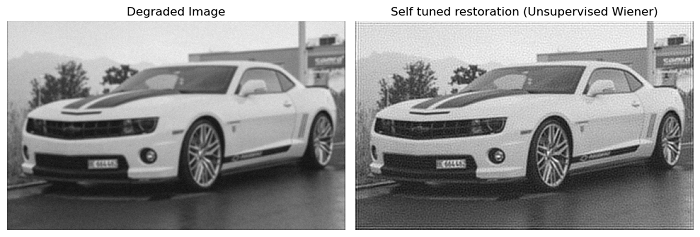
The following example restores an image obtained using the unsupervised Wiener deconvolution algorithm.

import numpy as np
import matplotlib.pyplot as plt
from skimage import color, io, restoration
from scipy.signal import convolve2d

# Load the astronaut image and convert it to grayscale
img = color.rgb2gray(io.imread('Images/Car_2.jpg'))

# Define a simple PSF (point spread function) 
psf = np.ones((5, 5)) / 25

# Simulate image degradation by convolving with the PSF
img = convolve2d(img, psf, 'same')

# Add Gaussian noise to the degraded image
rng = np.random.default_rng()
img += 0.1 * img.std() * rng.standard_normal(img.shape)

# Apply unsupervised Wiener deconvolution to restore the image
deconvolved_img, _ = restoration.unsupervised_wiener(img, psf)

# Create subplots for visualization
fig, axes = plt.subplots(1, 2, figsize=(10, 10))
ax1, ax2 = axes.ravel()

# Original Image
ax1.imshow(img, cmap='gray')
ax1.set_title('Degraded Image')
ax1.axis('off')

# Restored Image
ax2.imshow(deconvolved_img, cmap='gray')
ax2.set_title('Self tuned restoration (Unsupervised Wiener)')
ax2.axis('off')

plt.tight_layout()
plt.show()

Output

Print Page