Scikit Image - Tinting gray - scale images

---

---

Tinting an image refers to the process of adding a specific color or shade to an image to change its appearance. This process can be used to create artistic effects and highlight specific regions of an image.

Tinting grayscale images is a common image-processing technique for adding color to a black-and-white image. This process is typically achieved by manipulating the color channels of an image, often represented in the RGB color space.

In the RGB color space, a color image is represented as three 2D arrays corresponding to the Red (R), Green (G), and Blue (B) channels of the image. Each pixel in these arrays stores information about the intensity of that color channel at that particular location in the image. In grayscale images, these channels are usually the same, resulting in shades of gray.

Tinting the gray-scale images

One common method to achieve a tinted image involves adjusting the RGB channels by applying different scaling factors derived from the grayscale version of the image. For instance, by multiplying the green and blue channels by 0, it effectively removes those channels and leaves only the red channel. Likewise, when you eliminate the blue channel by multiplying it by 0, you're left with just the red and green channels, resulting in a yellow appearance as these two channels combine.

Example

The following example demonstrates how to use multipliers to artificially tint grayscale images in Python.

import matplotlib.pyplot as plt
from skimage import io 
from skimage import color
from skimage import img_as_float, img_as_ubyte

# Load a grayscale image
input_image = io.imread('Images/flowers.jpg', as_gray=True)
grayscale_image = img_as_float(input_image)

# Convert the grayscale image to a color image (RGB)
image = color.gray2rgb(grayscale_image)

# Define color multipliers for red and yellow tints
# Red tint: R=1, G=0, B=0
red_multiplier = [1, 0, 0] 

# Yellow tint: R=1, G=1, B=0
yellow_multiplier = [1, 1, 0]  

# Create a figure with two subplots, side by side
fig, (ax1, ax2) = plt.subplots(1, 2, figsize=(10, 5))

ax1.imshow(red_multiplier * image)
ax1.set_title('Red-tinted image')
ax1.set_axis_off()

# Display the yellow-tinted image in the second subplot
ax2.imshow(yellow_multiplier * image)
ax2.set_title('Yellow-tinted image')
ax2.set_axis_off()
plt.show()

Output

On executing the above program, you will get the following output −

Example

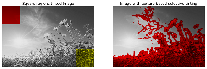
This example demonstrates how to use numpy slicing and fancy indexing to selectively tint the image regions.

from skimage.filters import rank
import matplotlib.pyplot as plt
from skimage import io 
from skimage import color
from skimage import img_as_float, img_as_ubyte
import numpy as np

# Load a grayscale image
input_image = io.imread('Images/flowers.jpg', as_gray=True)
grayscale_image = img_as_float(input_image)

# Convert the grayscale image to a color image (RGB)
image = color.gray2rgb(grayscale_image)

# Define square regions using slices for the first two dimensions.
top_left = (slice(100),) * 2
bottom_right = (slice(-100, None),) * 2

# Create a copy of the original image
sliced_image = image.copy()

# Define color multipliers for red and yellow tints
# Red tint: R=1, G=0, B=0
red_multiplier = [1, 0, 0] 

# Yellow tint: R=1, G=1, B=0
yellow_multiplier = [1, 1, 0]  

# Apply red multiplier to the top-left square region.
sliced_image[top_left] = image[top_left] * red_multiplier

# Apply yellow multiplier to the bottom-right square region.
sliced_image[bottom_right] = image[bottom_right] * yellow_multiplier

# Calculate a mask for regions with interesting texture using entropy filtering.
noisy = rank.entropy(img_as_ubyte(grayscale_image), np.ones((9, 9)))
textured_regions = noisy > 4.25

# Copy the original image for selective tinting based on texture.
masked_image = image.copy()

# Apply tinting to the textured regions.
masked_image[textured_regions, :] *= red_multiplier

# Create subplots for displaying the two selectively tinted images.
fig, (ax1, ax2) = plt.subplots(ncols=2, nrows=1, figsize=(12, 6))

ax1.imshow(sliced_image)
ax1.set_title('Square regions tinted Image')
ax1.set_axis_off()

ax2.imshow(masked_image)
ax2.set_title('Image with texture-based selective tinting')
ax2.set_axis_off()
plt.show()

Output

On executing the above program, you will get the following output −