- Computer Graphics - Home
- Computer Graphics Basics
- Computer Graphics Applications
- Graphics APIs and Pipelines
- Computer Graphics Maths
- Sets and Mapping
- Solving Quadratic Equations
- Computer Graphics Trigonometry
- Computer Graphics Vectors
- Linear Interpolation
- Computer Graphics Devices
- Cathode Ray Tube
- Raster Scan Display
- Random Scan Device
- Phosphorescence Color CRT
- Flat Panel Displays
- 3D Viewing Devices
- Images Pixels and Geometry
- Color Models
- Line Generation
- Line Generation Algorithm
- DDA Algorithm
- Bresenham's Line Generation Algorithm
- Mid-point Line Generation Algorithm
- Circle Generation
- Circle Generation Algorithm
- Bresenham's Circle Generation Algorithm
- Mid-point Circle Generation Algorithm
- Ellipse Generation Algorithm
- Polygon Filling
- Polygon Filling Algorithm
- Scan Line Algorithm
- Flood Filling Algorithm
- Boundary Fill Algorithm
- 4 and 8 Connected Polygon
- Inside Outside Test
- 2D Transformation
- 2D Transformation
- Transformation Between Coordinate System
- Affine Transformation
- Raster Methods Transformation
- 2D Viewing
- Viewing Pipeline and Reference Frame
- Window Viewport Coordinate Transformation
- Viewing & Clipping
- Point Clipping Algorithm
- Cohen-Sutherland Line Clipping
- Cyrus-Beck Line Clipping Algorithm
- Polygon Clipping Sutherland–Hodgman Algorithm
- Text Clipping
- Clipping Techniques
- Bitmap Graphics
- 3D Viewing Transformation
- 3D Computer Graphics
- Parallel Projection
- Orthographic Projection
- Oblique Projection
- Perspective Projection
- 3D Transformation
- Rotation with Quaternions
- Modelling and Coordinate Systems
- Back-face Culling
- Lighting in 3D Graphics
- Shadowing in 3D Graphics
- 3D Object Representation
- Represnting Polygons
- Computer Graphics Surfaces
- Visible Surface Detection
- 3D Objects Representation
- Computer Graphics Curves
- Computer Graphics Curves
- Types of Curves
- Bezier Curves and Surfaces
- B-Spline Curves and Surfaces
- Data Structures For Graphics
- Triangle Meshes
- Scene Graphs
- Spatial Data Structure
- Binary Space Partitioning
- Tiling Multidimensional Arrays
- Color Theory
- Colorimetry
- Chromatic Adaptation
- Color Appearance
- Antialiasing
- Ray Tracing
- Ray Tracing Algorithm
- Perspective Ray Tracing
- Computing Viewing Rays
- Ray-Object Intersection
- Shading in Ray Tracing
- Transparency and Refraction
- Constructive Solid Geometry
- Texture Mapping
- Texture Values
- Texture Coordinate Function
- Antialiasing Texture Lookups
- Procedural 3D Textures
- Reflection Models
- Real-World Materials
- Implementing Reflection Models
- Specular Reflection Models
- Smooth-Layered Model
- Rough-Layered Model
- Surface Shading
- Diffuse Shading
- Phong Shading
- Artistic Shading
- Computer Animation
- Computer Animation
- Keyframe Animation
- Morphing Animation
- Motion Path Animation
- Deformation Animation
- Character Animation
- Physics-Based Animation
- Procedural Animation Techniques
- Computer Graphics Fractals
Computer Graphics - 3D Transformation
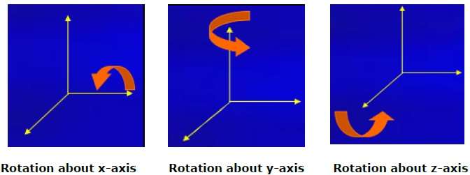
Rotation
3D rotation is not same as 2D rotation. In 3D rotation, we have to specify the angle of rotation along with the axis of rotation. We can perform 3D rotation about X, Y, and Z axes. They are represented in the matrix form as below −
$$R_{x}(\theta) = \begin{bmatrix} 1& 0& 0& 0\\ 0& cos\theta & −sin\theta& 0\\ 0& sin\theta & cos\theta& 0\\ 0& 0& 0& 1\\ \end{bmatrix} R_{y}(\theta) = \begin{bmatrix} cos\theta& 0& sin\theta& 0\\ 0& 1& 0& 0\\ −sin\theta& 0& cos\theta& 0\\ 0& 0& 0& 1\\ \end{bmatrix} R_{z}(\theta) =\begin{bmatrix} cos\theta & −sin\theta & 0& 0\\ sin\theta & cos\theta & 0& 0\\ 0& 0& 1& 0\\ 0& 0& 0& 1 \end{bmatrix}$$
The following figure explains the rotation about various axes −
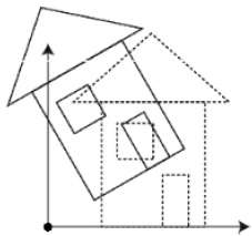
Scaling
You can change the size of an object using scaling transformation. In the scaling process, you either expand or compress the dimensions of the object. Scaling can be achieved by multiplying the original coordinates of the object with the scaling factor to get the desired result. The following figure shows the effect of 3D scaling −
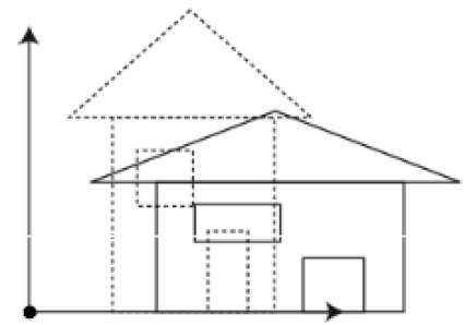
In 3D scaling operation, three coordinates are used. Let us assume that the original coordinates are (X, Y, Z), scaling factors are $(S_{X,} S_{Y,} S_{z})$ respectively, and the produced coordinates are (X, Y, Z). This can be mathematically represented as shown below −
$S = \begin{bmatrix} S_{x}& 0& 0& 0\\ 0& S_{y}& 0& 0\\ 0& 0& S_{z}& 0\\ 0& 0& 0& 1 \end{bmatrix}$
P = PS
$[{X}' \:\:\: {Y}' \:\:\: {Z}' \:\:\: 1] = [X \:\:\:Y \:\:\: Z \:\:\: 1] \:\: \begin{bmatrix} S_{x}& 0& 0& 0\\ 0& S_{y}& 0& 0\\ 0& 0& S_{z}& 0\\ 0& 0& 0& 1 \end{bmatrix}$
$ = [X.S_{x} \:\:\: Y.S_{y} \:\:\: Z.S_{z} \:\:\: 1]$
Shear
A transformation that slants the shape of an object is called the shear transformation. Like in 2D shear, we can shear an object along the X-axis, Y-axis, or Z-axis in 3D.
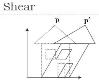
As shown in the above figure, there is a coordinate P. You can shear it to get a new coordinate P', which can be represented in 3D matrix form as below −
$Sh = \begin{bmatrix} 1 & sh_{x}^{y} & sh_{x}^{z} & 0 \\ sh_{y}^{x} & 1 & sh_{y}^{z} & 0 \\ sh_{z}^{x} & sh_{z}^{y} & 1 & 0 \\ 0 & 0 & 0 & 1 \end{bmatrix}$
P = P Sh
$X = X + Sh_{x}^{y} Y + Sh_{x}^{z} Z$
$Y' = Sh_{y}^{x}X + Y +sh_{y}^{z}Z$
$Z' = Sh_{z}^{x}X + Sh_{z}^{y}Y + Z$
Transformation Matrices
Transformation matrix is a basic tool for transformation. A matrix with n x m dimensions is multiplied with the coordinate of objects. Usually 3 x 3 or 4 x 4 matrices are used for transformation. For example, consider the following matrix for various operation.
| $T = \begin{bmatrix} 1& 0& 0& 0\\ 0& 1& 0& 0\\ 0& 0& 1& 0\\ t_{x}& t_{y}& t_{z}& 1\\ \end{bmatrix}$ | $S = \begin{bmatrix} S_{x}& 0& 0& 0\\ 0& S_{y}& 0& 0\\ 0& 0& S_{z}& 0\\ 0& 0& 0& 1 \end{bmatrix}$ | $Sh = \begin{bmatrix} 1& sh_{x}^{y}& sh_{x}^{z}& 0\\ sh_{y}^{x}& 1 & sh_{y}^{z}& 0\\ sh_{z}^{x}& sh_{z}^{y}& 1& 0\\ 0& 0& 0& 1 \end{bmatrix}$ |
| Translation Matrix | Scaling Matrix | Shear Matrix |
| $R_{x}(\theta) = \begin{bmatrix} 1& 0& 0& 0\\ 0& cos\theta & -sin\theta& 0\\ 0& sin\theta & cos\theta& 0\\ 0& 0& 0& 1\\ \end{bmatrix}$ | $R_{y}(\theta) = \begin{bmatrix} cos\theta& 0& sin\theta& 0\\ 0& 1& 0& 0\\ -sin\theta& 0& cos\theta& 0\\ 0& 0& 0& 1\\ \end{bmatrix}$ | $R_{z}(\theta) = \begin{bmatrix} cos\theta & -sin\theta & 0& 0\\ sin\theta & cos\theta & 0& 0\\ 0& 0& 1& 0\\ 0& 0& 0& 1 \end{bmatrix}$ |
| Rotation Matrix | ||