Computer Graphics - Polygon Filling Algorithm

---

---

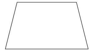
Polygon is an ordered list of vertices as shown in the following figure. For filling polygons with particular colors, you need to determine the pixels falling on the border of the polygon and those which fall inside the polygon. In this chapter, we will see how we can fill polygons using different techniques.

Scan Line Algorithm

This algorithm works by intersecting scanline with polygon edges and fills the polygon between pairs of intersections. The following steps depict how this algorithm works.

Step 1 − Find out the Ymin and Ymax from the given polygon.

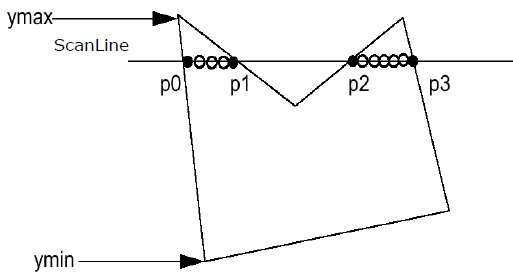
Step 2 − ScanLine intersects with each edge of the polygon from Ymin to Ymax. Name each intersection point of the polygon. As per the figure shown above, they are named as p0, p1, p2, p3.

Step 3 − Sort the intersection point in the increasing order of X coordinate i.e. (p0, p1), (p1, p2), and (p2, p3).

Step 4 − Fill all those pair of coordinates that are inside polygons and ignore the alternate pairs.

Flood Fill Algorithm

Sometimes we come across an object where we want to fill the area and its boundary with different colors. We can paint such objects with a specified interior color instead of searching for particular boundary color as in boundary filling algorithm.

Instead of relying on the boundary of the object, it relies on the fill color. In other words, it replaces the interior color of the object with the fill color. When no more pixels of the original interior color exist, the algorithm is completed.

Once again, this algorithm relies on the Four-connect or Eight-connect method of filling in the pixels. But instead of looking for the boundary color, it is looking for all adjacent pixels that are a part of the interior.

Boundary Fill Algorithm

The boundary fill algorithm works as its name. This algorithm picks a point inside an object and starts to fill until it hits the boundary of the object. The color of the boundary and the color that we fill should be different for this algorithm to work.

In this algorithm, we assume that color of the boundary is same for the entire object. The boundary fill algorithm can be implemented by 4-connected pixels or 8-connected pixels.

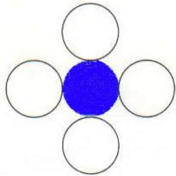
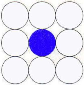
4-Connected Polygon

In this technique 4-connected pixels are used as shown in the figure. We are putting the pixels above, below, to the right, and to the left side of the current pixels and this process will continue until we find a boundary with different color.

Algorithm

Step 1 − Initialize the value of seed point (seedx, seedy), fcolor and dcol.

Step 2 − Define the boundary values of the polygon.

Step 3 − Check if the current seed point is of default color, then repeat the steps 4 and 5 till the boundary pixels reached.

If getpixel(x, y) = dcol then repeat step 4 and 5

Step 4 − Change the default color with the fill color at the seed point.

setPixel(seedx, seedy, fcol)

Step 5 − Recursively follow the procedure with four neighborhood points.

FloodFill (seedx  1, seedy, fcol, dcol)
FloodFill (seedx + 1, seedy, fcol, dcol)
FloodFill (seedx, seedy - 1, fcol, dcol)
FloodFill (seedx  1, seedy + 1, fcol, dcol)

Step 6 − Exit

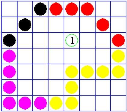
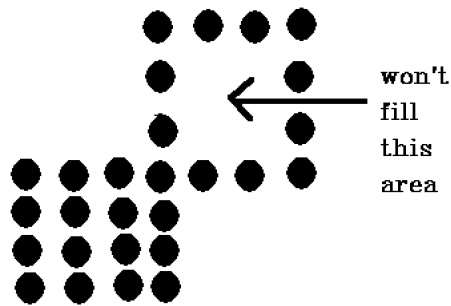
There is a problem with this technique. Consider the case as shown below where we tried to fill the entire region. Here, the image is filled only partially. In such cases, 4-connected pixels technique cannot be used.

8-Connected Polygon

In this technique 8-connected pixels are used as shown in the figure. We are putting pixels above, below, right and left side of the current pixels as we were doing in 4-connected technique.

In addition to this, we are also putting pixels in diagonals so that entire area of the current pixel is covered. This process will continue until we find a boundary with different color.

Algorithm

Step 1 − Initialize the value of seed point (seedx, seedy), fcolor and dcol.

Step 2 − Define the boundary values of the polygon.

Step 3 − Check if the current seed point is of default color then repeat the steps 4 and 5 till the boundary pixels reached

If getpixel(x,y) = dcol then repeat step 4 and 5

Step 4 − Change the default color with the fill color at the seed point.

setPixel(seedx, seedy, fcol)

Step 5 − Recursively follow the procedure with four neighbourhood points

FloodFill (seedx  1, seedy, fcol, dcol)
FloodFill (seedx + 1, seedy, fcol, dcol)
FloodFill (seedx, seedy - 1, fcol, dcol)
FloodFill (seedx, seedy + 1, fcol, dcol)
FloodFill (seedx  1, seedy + 1, fcol, dcol)
FloodFill (seedx + 1, seedy + 1, fcol, dcol)
FloodFill (seedx + 1, seedy - 1, fcol, dcol)
FloodFill (seedx  1, seedy - 1, fcol, dcol)

Step 6 − Exit

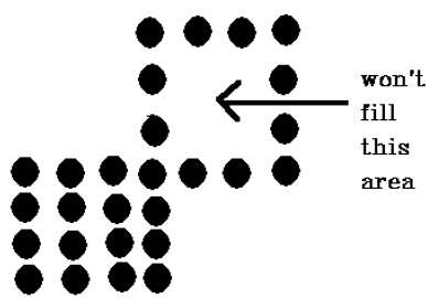
The 4-connected pixel technique failed to fill the area as marked in the following figure which wont happen with the 8-connected technique.

Inside-outside Test

This method is also known as counting number method. While filling an object, we often need to identify whether particular point is inside the object or outside it. There are two methods by which we can identify whether particular point is inside an object or outside.

• Odd-Even Rule
• Nonzero winding number rule

Odd-Even Rule

In this technique, we will count the edge crossing along the line from any point (x,y) to infinity. If the number of interactions is odd, then the point (x,y) is an interior point; and if the number of interactions is even, then the point (x,y) is an exterior point. The following example depicts this concept.

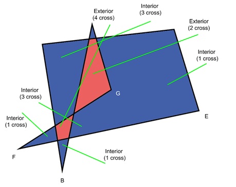
From the above figure, we can see that from the point (x,y), the number of interactions point on the left side is 5 and on the right side is 3. From both ends, the number of interaction points is odd, so the point is considered within the object.

Nonzero Winding Number Rule

This method is also used with the simple polygons to test the given point is interior or not. It can be simply understood with the help of a pin and a rubber band. Fix up the pin on one of the edge of the polygon and tie-up the rubber band in it and then stretch the rubber band along the edges of the polygon.

When all the edges of the polygon are covered by the rubber band, check out the pin which has been fixed up at the point to be test. If we find at least one wind at the point consider it within the polygon, else we can say that the point is not inside the polygon.

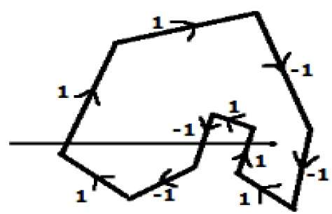
In another alternative method, give directions to all the edges of the polygon. Draw a scan line from the point to be test towards the left most of X direction.

• Give the value 1 to all the edges which are going to upward direction and all other -1 as direction values.

• Check the edge direction values from which the scan line is passing and sum up them.

• If the total sum of this direction value is non-zero, then this point to be tested is an interior point, otherwise it is an exterior point.

• In the above figure, we sum up the direction values from which the scan line is passing then the total is 1 1 + 1 = 1; which is non-zero. So the point is said to be an interior point.