Smooth-Layered Model in Computer Graphics

---

---

We have explained the concept of specularity in the previous chapter. Specularity plays a key role in smooth-layered models. This model is ideal for materials like plastics, polished wood, and glossy tiles. It uses the principles of the Fresnel equations to handle surface reflections and scattering within subsurfaces.

Read this chapter to learn the Smooth-Layered Model. Here we will cover the basics, the mathematical foundations, and examples of how it can be applied in computer graphics.

What is Smooth-Layered Model?

The Smooth-Layered Model is designed for materials having both specular and matte reflections. Such materials include polished wood, plastic, and ceramics. In these materials, light reflects off the surface and also scatters within the subsurface.

The specular reflection is done by the Fresnel equations. Subsurface scattering affects the light that is not reflected directly from the surface. The model handles both components to create a realistic appearance.

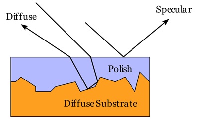
For example, when looking at polished tiles, we will see reflections that appear sharp but become blurry and diffuse in certain areas. This happens because light interacts with both the surface and the underlying layers.

Basic Equation of the Smooth-Layered Model

The smooth-layered model combines both matte and specular reflection terms. The traditional Lambertian-specular model for matte and specular components can be expressed using the following formula −

$$\mathrm{\rho(\theta,\: \phi,\: \theta',\: \phi',\: \lambda) \:=\: R_f(\theta)\: \rho_s(\theta,\: \phi,\: \theta',\: \phi') \:+\: \frac{R_d(\lambda)}{\pi}}$$

Where,

• R_d(λ) − This represents the hemispherical reflectance of the matte term.
• R_s − This is the specular reflectance.
• ρ_s − This is the normalized specular BRDF (Bidirectional Reflectance Distribution Function).

This equation models how light reflects and scatters in materials like polished wood. For many applications, setting R_d(λ) + R_s ≤ 1. This ensures that energy is conserved.

Adjusting the Matte and Specular Tradeoff

The matte and specular reflections change with the viewing angle. The smooth-layered model adjusts these proportions to achieve the desired look.

For example, the matte appearance decreases as the specular reflectance increases with the viewing angle. A common adjustment is made by dampening R_d(λ) as R_s increases −

$$\mathrm{\rho(\theta,\: \phi,\: \theta',\: \phi',\: \lambda) \:=\: R_f(\theta)\: \rho_s(\theta,\: \phi,\: \theta',\: \phi') \:+\: \frac{R_d(\lambda)(1 \:-\: R_f(\theta))}{\pi}}$$

Here, R_f(θ) is the Fresnel reflectance for a polish-air interface. This equation works well for most materials but has some limitations. It is not reciprocal and might not produce correct results for certain rendering methods.

Coupled Model for Specular and Matte Components

We also learnt a little in the last article. The coupled model improves upon the traditional smooth-layered model by keeping the matte and specular components consistent. It achieves energy conservation and reciprocity.

This model shows that as the specular reflection increases with the viewing angle, the matte reflection decreases proportionally. It uses the following equation −

$$\mathrm{\rho(\theta,\: \phi,\: \theta',\: \phi',\: \lambda) \:=\: R_f(\theta)\: \rho_s(\theta,\: \phi,\: \theta',\: \phi') \:+\: k R_m(\lambda) \left[ 1 \:-\: R_f(\theta) \right] \left[ 1 \:-\: R_f(\theta') \right]}$$

Where,

• k − A constant used for balancing the reflection components.
• R_m(λ) − The matte reflectance parameter.

This equation is more accurate for materials with a clear dielectric surface, like a polished wooden surface. The coupled model effectively simulates the change in appearance with different viewing angles.

What is Fresnel Reflectance?

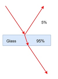
From the glossy and glass materials, we know that the Fresnel equations are useful for calculating the reflectance of smooth surfaces. These equations describe how light behaves at the interface of two different media.

In the coupled model, R_f(θ) is the Fresnel reflectance for a given angle θ. This component helps simulate the shiny appearance of the surface. It affects how much light is reflected or transmitted through the surface.

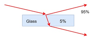
For example, when viewing a polished tile from a steep angle, the reflections appear sharp and strong. As the viewing angle becomes more perpendicular, the reflections become softer and less intense. The Fresnel equations is useful to achieve these variations in intensity and sharpness.

Example: Using the Smooth-Layered Model for Polished Tiles

The polished tiles are a good example to demonstrate the smooth-layered model. When light hits a polished tile, some of it reflects off the surface, creating a specular reflection. The rest of the light penetrates the surface, scatters within the material, and then exits, forming the matte reflection.

In the smooth-layered model, the specular reflection is calculated using the Fresnel equations. The matte reflection is handled by a simple function that depends on the viewing angle and the wavelength of light. The model uses a term f(θ), which can be expressed as:

$$\mathrm{f(\theta)\: \propto\: \left( 1 \:-\: (1 \:-\: \cos \theta)^5 \right)}$$

By combining these terms, the model accurately simulates how polished tiles reflect light under different conditions.

Benefits and Limitations of the Smooth-Layered Model

The smooth-layered model has several benefits. It provides realistic reflections for materials like polished wood or ceramics. It is easy to implement and does not require detailed subsurface information. However, it has limitations as well.

The model assumes that the surface is smooth. If the surface has bumps or roughness, the reflection will not be accurate. For such surfaces, a rough-layered model should be used instead.

Conclusion

In this chapter, we have explained the smooth-layered model for reflection in computer graphics. We covered its basics and how it works for materials like polished wood and plastic. We then covered the mathematical foundations and Fresnel equations used in the model.

We also understand the coupled model in detail along with its balancing style for the matte and specular components. Finally, we looked at an example of how the model is applied to polished tiles.