Tiling Multi-dimensional Arrays in Computer Graphics

---

---

Tiling of multidimensional arrays is one of the key methods to enhance performance. Tiling means optimizing the use of the memory hierarchy by organizing data in such a way that it is accessed more efficiently. Read this chapter to understand the basic concept of tiling, its importance, and how it is applied in both 2D and 3D arrays.

Tiling Multi-dimensional Arrays

Memory is accessed in blocks, and data that is stored closer together is typically accessed faster. In computer graphics, large datasets such as images, volumes, or textures are often represented as multidimensional arrays. A problem may come when these arrays are stored in a poor memory locality formation. Means, adjacent elements in the array are not stored near each other in memory. It can cause performance issues when the system has to jump around in memory to access the necessary data.

Tiling (also known as bricking) solves this problem by breaking the array into smaller blocks or tiles. These tiles are stored contiguously in memory. It makes the access to adjacent data elements faster and more efficient. This technique is particularly useful in modern architectures, where memory hierarchies play a significant role in determining the speed of data access.

Traditional Memory Layout for 2D Arrays

Before understanding the idea of tiling, let us see the traditional memory layout for a 2D array. In a simple 2D array with dimensions N_x × N_y, the data is usually stored as a 1D array. The 2D index (x, y) is mapped to a 1D index using the following formula:

$$\mathrm{\text{Index} \:=\: x \:+\: N_x\: \times\: y}$$

This formula works fine if the system is processing the data row by row. However, if the system needs to process the data column by column, this layout becomes inefficient. In this case, two adjacent elements in a column are separated by N_x elements in memory, which can lead to poor memory locality and cache performance.

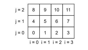
In this example, where an array of size 4 × 3 is stored linearly in memory. Accessing elements in the same row is fast because they are stored next to each other. However, accessing elements in the same column requires jumping over several elements, leading to inefficient memory usage.

Tiling for Better Memory Locality

To solve the problem of poor memory locality, we can divide the array into smaller tiles. Each tile contains a small block of the array, and these tiles are stored contiguously in memory. This ensures that when the system accesses data within a tile, it does so efficiently.

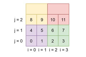
For example, here in tiled layout of the same 4 × 3 array, where each tile is 2 × 2. The elements within each tile are stored together, improving both row and column access performance. The result is better memory locality. The system can access adjacent elements in both rows and columns more quickly.

Choosing the Tile Size

Another important factor is choosing the appropriate tile size. The size of the tiles should match the size of the memory unit on the machine.

For example, if the system has a cache line size of 128 bytes and each data element is 2 bytes (16-bit), then a tile of size 8 × 8 fits perfectly into a cache line.

However, for systems using 32-bit floating-point numbers (4 bytes), the ideal tile size might be 6 × 6 or 5 × 5, depending on the architecture.

One-Level Tiling for 2D Arrays

Let us now consider how to implement one-level tiling for a 2D array. In this case, the array is divided into square tiles, and each tile is stored contiguously in memory.

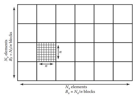
Breaking Down the Array into Tiles

Assume we have an array of size N_x × N_y, and we want to decompose it into tiles of size n × n. The number of tiles required in each dimension is given by:

$$\mathrm{B_x \:=\: \frac{N_x}{n}}$$

$$\mathrm{B_y \:=\: \frac{N_y}{n}}$$

Where B_x and B_y are the number of tiles in the x and y dimensions, respectively.

Indexing in a Tiled Array

To access an element (x, y) in the tiled array, we first need to determine which tile contains the element and then compute the position of the element within the tile.

The tile indices are given by −

$$\mathrm{b_x \:=\: \frac{x}{n}}$$

$$\mathrm{b_y \:=\: \frac{y}{n}}$$

Here, ÷ represents integer division. The offsets within the tile are −

$$\mathrm{x' \:=\: x \mod n}$$

$$\mathrm{y' \:=\: y \mod n}$$

Finally, the 1D index of the element in the tiled array is computed as −

$$\mathrm{\text{Index} \:=\: n^2\: \times \:(B_x \: \times\: b_y \:+\: b_x) \:+\: (y'\: \times\: n \:+\: x')}$$

This formula states that each element is accessed efficiently within its tile. The system can quickly calculate the tile and the position within the tile, leading to improved memory locality and performance.

Two-Level Tiling for 3D Arrays

For larger datasets, such as 3D arrays, two-level tiling can be used to further optimize memory usage. In this case, the array is divided into macrobricks, and each macrobrick contains multiple smaller tiles (or bricks).

Example of Two-Level Tiling

Consider a 3D array with dimensions 40 × 20 × 19. We can decompose this array into macrobricks of size 2 × 2 × 2, where each macrobrick contains bricks of size 5 × 5 × 5. This results in a hierarchical tiling structure that optimizes memory access in all three dimensions.

Indexing in a Two-Level Tiled Array

The indexing for a two-level tiled array is more complex but follows the same principles as one-level tiling. The array is first divided into macrobricks, and each macrobrick is then further divided into smaller bricks.

The formula for accessing an element (x, y, z) in a two-level tiled array is −

$$\mathrm{\text{Index} \:=\: F_x(x) \:+\: F_y(y) \:+\: F_z(z)}$$

Where F_x(x), F_y(y), and F_z(z) are the functions that compute the index of the element based on its position in the X, Y, and Z dimensions, respectively. These functions take into account both the macrobrick and brick sizes. It is ensuring efficient access to the element in memory.

Conclusion

In this chapter, we covered the concept of tiling multidimensional arrays in computer graphics. We highlighted the traditional memory layout for 2D arrays and the problems it can cause with memory locality. We then introduced the concept of tiling and explained how it improves memory access by storing adjacent data elements together.

We also covered the process of one-level tiling for 2D arrays, including how to index elements within a tiled array. Finally, we looked at two-level tiling for 3D arrays.