Rough-Layered Model in Computer Graphics

---

---

The rough-layered model handles surfaces that are not perfectly smooth. It can represent common materials such as metal, plastic, and other rough surfaces. The model holds the features like energy conservation, anisotropy, and intuitive parameters for easier implementation.

In this chapter, we will explain the Rough-Layered Model in detail and also its basic concepts, providing examples to demonstrate its application for a better understanding.

What is Rough-Layered Model?

The rough-layered model extends the concept of the smooth-layered model to handle rough surfaces. For surfaces that are not perfectly smooth, reflections appear more blurred or diffused. This model shows a spread in the specular component. That light reflects in multiple directions rather than a single direction.

Rough surfaces are challenging to simulate because they require additional parameters to capture the scattering behavior. The Rough-Layered Model simplifies this process by using a Fresnel-weighted, Phong-style cosine lobe that is anisotropic. It can handle materials like brushed metal or rough plastic, where light reflects differently based on the surface's orientation.

Characteristics of the Rough-Layered Model

Let us see some characteristics of a rough-layered surface that will scatter light in a way that depends on the roughness of the surface.

• Plausibility − The model obeys energy conservation and reciprocity. This means that the energy of the incoming light is equal to the energy of the outgoing light. It shows realistic reflections.
• Anisotropy − It models simple anisotropy, which is the variation in reflectance based on the direction of the surface. For example, brushed metal surfaces reflect light differently along different axes.
• Intuitive Parameters − The model uses parameters like the roughness values n_u and n_v for different directions. This makes it easy to set up materials and get the desired effect.
• Fresnel Behavior − The specular component of the reflection increases as the incident angle decreases. This means that surfaces appear shinier at steep viewing angles.
• Non-Lambertian Diffuse Term − The diffuse component of the reflection is non-Lambertian, meaning it does not scatter light equally in all directions. This ensures energy conservation even in the presence of Fresnel behavior.
• Monte Carlo Friendliness − The model has a probability density function that allows straightforward Monte Carlo sampling for rendering.

For these characteristics, the rough-layered model are versatile and suitable for different surface types.

Mathematical Formulation of the Rough-Layered Model

The Rough-Layered Model decomposes the BRDF (Bidirectional Reflectance Distribution Function) into two parts: the specular component and the diffuse component.

This is represented using the following formula −

$$\mathrm{\rho(k_1,\: k_2) \:=\: \rho_s(k_1,\: k_2) \:+\: \rho_d(k_1,\: k_2)}$$

Where,

• ρ_s(k₁,k₂) − This is the specular reflection component. It accounts for the mirror-like reflection on the surface.
• ρ_d(k₁,k₂) − This is the diffuse reflection component. It handles the light that is scattered in many directions.

The specular component can be represented using a Phong-style cosine lobe that incorporates anisotropy. The equation for this is given as −

$$\mathrm{\rho(k_1,\: k_2) \:=\: \frac{(n_u \:+\: 1)(n_v \:+\: 1)}{8\pi} \frac{(n \:\cdot\: h)^{n_u} \cos^2 \phi \:+\: n_v \sin^2 \phi}{(h \:\cdot\: k_i) \max(\cos \:\theta_i,\: \cos \theta_o)} F(k_i,\: h)}$$

In this equation −

• n_u and n_v are roughness parameters in two different directions.
• h is the halfway vector between the incoming and outgoing directions.
• is the azimuthal angle, which controls the directionality of the reflection.
• F(k_i⋅h) is the Fresnel term that controls the amount of light reflected based on the angle of incidence.

Example: Using the Rough-Layered Model for Metallic Surfaces

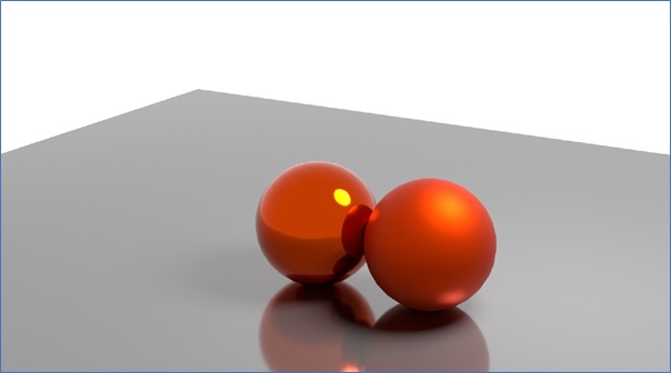
The Rough-Layered Model is especially useful for representing metallic surfaces. Metals like gold or brushed aluminum reflect light in a way that depends on the roughness and anisotropy of the surface. As the roughness parameters n_u and n_v change, the appearance of the surface changes from a rough and also diffused reflection to a sharper.

For example, consider a set of metallic spheres rendered using the rough-layered model. As the roughness values n_u and n_v increase, the reflection on the surface becomes more blurred. This indicates a rougher surface. Conversely, when the values decrease, the surface appears shinier and more reflective, like a polished metal.

The following equation captures the specular behavior of such surfaces −

$$\mathrm{F(k_i,\: h) \:=\: R_s \:+\: (1 \:+\: R_s) \left( 1 \:-\: (k_i \:\cdot\: h) \right)^5}$$

This is Schlick’s approximation of the Fresnel equation, where R_s is the material’s reflectance at normal incidence. It controls how much light is reflected based on the angle between the incoming light and the surface normal.

Implementation of the Rough-Layered Model

The Rough-Layered Model is implemented using the anisotropic Phong-style specular BRDF. This model can be easily incorporated into rendering engines. It helps in flexible material setups. For example, by adjusting the n_u and n_v parameters, users can control the roughness of the surface in two different directions.

The diffuse component can also be modified to ensure energy conservation. This is done by using a non-Lambertian diffuse term that matches the directional pattern of the specular component. This ensures that no energy is lost in the scattering process.

Benefits and Limitations of the Rough-Layered Model

We have understood that the rough-layered model offers several benefits for rendering complex surfaces. It is physically plausible and obeys energy conservation. It can represent anisotropic surfaces accurately and is easy to use. However, there are some limitations.

The model assumes that the surface is relatively smooth. For highly irregular surfaces, a more complex model may be required.

The model also requires careful tuning of parameters like n_u, n_v and R_s to get the desired visual effects. This can be challenging for beginners.

Conclusion

In this chapter, we covered the rough-layered model for reflection in computer graphics. We explained its basic concepts and characteristics. We then discussed the mathematical formulation, including the specular and diffuse components.

We also presented examples of how the model is used for metallic surfaces with varying roughness. Finally, we understood the benefits and limitations of the Rough-Layered Model.