Representing Polygons in Computer Graphics

---

---

Polygons are shapes made of straight lines, and their representation in computer graphics determines how we can manipulate and fill areas inside these shapes. We will see some basic ideas about polygons before getting into the methods used to represent them in graphic systems. Read this chapter to learn how polygons can be represented in computer graphics.

What are Polygons?

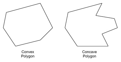
A polygon is a closed shape formed by connecting straight lines. The points where two lines meet are called vertices. Polygons come in different forms such as concave polygons and convex polygons.

• Convex polygons have all their interior angles less than 180 degrees.
• Concave polygons have one or more interior angles greater than 180 degrees.

Let us see how these polygons can be represented in a computer system.

Coding Polygons in a Computer System

When we represent polygons in a system, we need to consider how they will be shown and manipulated. Suppose we have a polygon, and we want to display it inside the system. To achieve this, we need to think about how we will design the code based on the shape of the polygon. Once we understand this, we can write code to represent it.

There are several approaches to represent polygons inside computers. Three such mostly used methods are:

• Polygon Drawing Primitive Approach
• Trapezoid Primitive Approach
• Line and Point Approach

Let us go over each approach in detail to understand how polygons are represented in a computer graphic system.

Polygon Drawing Primitive Approach

The Polygon Drawing Primitive Approach allows polygons to be drawn directly as shapes.

In this method, polygons are saved as one unit in the system. For example, suppose we are using software like Photoshop or Corel Draw. When we click on the polygon tool and select the number of sides, the software generates a polygon. We might ask it to create a polygon with 5 sides. The software does not ask you for more information, like the length of each side or the exact coordinates. It simply draws a polygon of 5 sides.

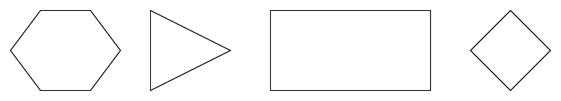
This approach mainly deals with regular polygons, where:

• All sides of the polygon are of equal length.
• All angles inside the polygon are equal.

If you stretch or shrink the polygon, the system adjusts it proportionally. The polygon is treated as one complete unit. So, whether it is a pentagon, hexagon, or any other regular polygon, it can be drawn directly without asking for too many details.

Trapezoid Primitive Approach

The second method is the Trapezoid Primitive Approach. This approach gets its name from the shape trapezoid. A trapezoid (or trapezium) is a shape with four sides, where one pair of sides is parallel.

In this method, polygons are broken down into trapezoids for representation. The system converts the polygon into a series of trapezoids using two scanlines and two line segments. The scanlines run parallel to each other, while the line segments form the sides of the polygon.

Example of Trapezoid Representation

Imagine we need to represent a polygon with n sides. The system will start by drawing parallel scanlines across the polygon. Then, it looks at two sides of the polygon and uses them to create trapezoids between the scanlines.

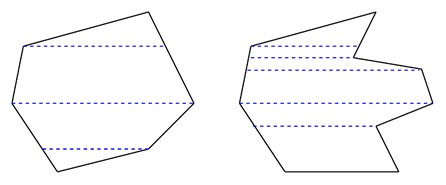
The polygon’s top and bottom lines are traced by the scanlines, while the side lines form the edges of the trapezoid. The system keeps stepping down from one line to the next, creating trapezoids as it goes along. These trapezoids are then filled with color or texture.

Each time the scanline reaches the next point on the polygon, it creates a new trapezoid. This method helps in raster graphics, where the system needs to fill the shape with pixels. Using trapezoids makes it easier for the system to fill in the areas between the lines.

Line and Point Approach

The third method is the Line and Point Approach. This method is used on devices that do not directly support polygons. In some graphic systems, there may be no built-in tools to create polygons. In such cases, we use this approach to represent polygons through lines and points.

In the Line and Point Approach, polygons are created by combining lines and points. However, there is a limitation with this approach. We cannot simply give the system a bunch of line commands and expect it to draw a polygon. This is because the system cannot tell which lines are part of the polygon and which lines are not.

Overcoming the Limitation

To solve this problem, a new command is used in the display file. This new command, called an opcode. This specifies how many line segments are part of the polygon.

For example, if a polygon has five sides, the opcode will say there are five line segments. The system will then take the information from the opcode and connect the lines to form the polygon.

This command also helps the system recognize the correct lines to connect. Without this, there would be confusion, as the system might join lines that are not supposed to form part of the polygon. By using opcodes, the system knows how many lines there are and can correctly draw the polygon.

Example of the Line and Point Approach

Let us see the same polygon with this point line approach. Here we must know the points and their coordinates, then the lines to connect these coordinates.

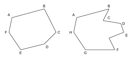
For example, for the first polygon, there are 6 points and they must have their coordinates. The lines are AB, BC, CD, DE, EF. Similarly for the next one as well. The rostering device will plot these points and lines to draw the polygons.

Conclusion

There are three different approaches for representing polygons in computer graphics. Polygon Drawing Primitive Approach, which draws polygons as single units, often used in software where regular polygons are created with equal side lengths and angles.

The trapezoid primitive approach which draw polygons by broken down into trapezoids using scanlines and line segments. It is helpful for systems that need to fill polygons with pixels.

And finally, the line and point approach, which is used on devices that do not directly support polygons. It uses opcodes to specify how many line segments form a polygon.