- Computer Graphics - Home
- Computer Graphics Basics
- Computer Graphics Applications
- Graphics APIs and Pipelines
- Computer Graphics Maths
- Sets and Mapping
- Solving Quadratic Equations
- Computer Graphics Trigonometry
- Computer Graphics Vectors
- Linear Interpolation
- Computer Graphics Devices
- Cathode Ray Tube
- Raster Scan Display
- Random Scan Device
- Phosphorescence Color CRT
- Flat Panel Displays
- 3D Viewing Devices
- Images Pixels and Geometry
- Color Models
- Line Generation
- Line Generation Algorithm
- DDA Algorithm
- Bresenham's Line Generation Algorithm
- Mid-point Line Generation Algorithm
- Circle Generation
- Circle Generation Algorithm
- Bresenham's Circle Generation Algorithm
- Mid-point Circle Generation Algorithm
- Ellipse Generation Algorithm
- Polygon Filling
- Polygon Filling Algorithm
- Scan Line Algorithm
- Flood Filling Algorithm
- Boundary Fill Algorithm
- 4 and 8 Connected Polygon
- Inside Outside Test
- 2D Transformation
- 2D Transformation
- Transformation Between Coordinate System
- Affine Transformation
- Raster Methods Transformation
- 2D Viewing
- Viewing Pipeline and Reference Frame
- Window Viewport Coordinate Transformation
- Viewing & Clipping
- Point Clipping Algorithm
- Cohen-Sutherland Line Clipping
- Cyrus-Beck Line Clipping Algorithm
- Polygon Clipping Sutherland–Hodgman Algorithm
- Text Clipping
- Clipping Techniques
- Bitmap Graphics
- 3D Viewing Transformation
- 3D Computer Graphics
- Parallel Projection
- Orthographic Projection
- Oblique Projection
- Perspective Projection
- 3D Transformation
- Rotation with Quaternions
- Modelling and Coordinate Systems
- Back-face Culling
- Lighting in 3D Graphics
- Shadowing in 3D Graphics
- 3D Object Representation
- Represnting Polygons
- Computer Graphics Surfaces
- Visible Surface Detection
- 3D Objects Representation
- Computer Graphics Curves
- Computer Graphics Curves
- Types of Curves
- Bezier Curves and Surfaces
- B-Spline Curves and Surfaces
- Data Structures For Graphics
- Triangle Meshes
- Scene Graphs
- Spatial Data Structure
- Binary Space Partitioning
- Tiling Multidimensional Arrays
- Color Theory
- Colorimetry
- Chromatic Adaptation
- Color Appearance
- Antialiasing
- Ray Tracing
- Ray Tracing Algorithm
- Perspective Ray Tracing
- Computing Viewing Rays
- Ray-Object Intersection
- Shading in Ray Tracing
- Transparency and Refraction
- Constructive Solid Geometry
- Texture Mapping
- Texture Values
- Texture Coordinate Function
- Antialiasing Texture Lookups
- Procedural 3D Textures
- Reflection Models
- Real-World Materials
- Implementing Reflection Models
- Specular Reflection Models
- Smooth-Layered Model
- Rough-Layered Model
- Surface Shading
- Diffuse Shading
- Phong Shading
- Artistic Shading
- Computer Animation
- Computer Animation
- Keyframe Animation
- Morphing Animation
- Motion Path Animation
- Deformation Animation
- Character Animation
- Physics-Based Animation
- Procedural Animation Techniques
- Computer Graphics Fractals
Ellipse Generation Algorithm in Computer Graphics
Midpoint algorithms are particularly valuable in rendering ellipses accurately on a pixel grid. In this chapter, we will see the basic concept of the ellipse drawing algorithm, explain how it works, and provide a detailed example for a better understanding.
Midpoint Ellipse Drawing Algorithm
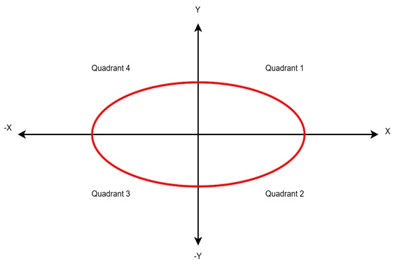
The Midpoint Ellipse Algorithm is used for scan converting an ellipse whose center point is at the origin with its major and minor axes aligned to the coordinate axes. It is an incremental approach, much like the Midpoint Circle Algorithm, and is based on the symmetry of the ellipse. An ellipse can be divided into four quadrants due to its symmetry, allowing us to calculate points for just one quadrant and mirror them to the others.
This algorithm is efficient because it works in an incremental manner. Here only additions or subtractions are used in decision-making. One can skip complex operations like multiplication or square roots.
Basic Concepts of Midpoint Ellipse Drawing Algorithm
To understand the midpoint ellipse algorithm, we need to be familiar with the equation of an ellipse −
$$\mathrm{\frac{x^2}{a^2} \:+\: \frac{y^2}{b^2} \:=\: 1}$$
Where,
- a is the semi-major axis (the horizontal radius)
- b is the semi-minor axis (the vertical radius)
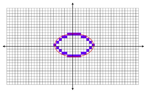
The goal of the algorithm is to plot the points of this ellipse by using the incremental approach to determine which pixel is closer to the actual ellipse boundary. We achieve this by calculating the midpoint between two potential pixels and checking if this midpoint lies inside or outside the ellipse.
Let's now understand how the Midpoint Ellipse Drawing Algorithm works.
Symmetry and Quadrants
Since the ellipse has four-way symmetry, the algorithm only computes points for the first quadrant and mirrors them to the remaining three quadrants.
Slope and Decision Parameter
The slope of the curve is needed for determining the decision point. Initially, the starting point is at (0, b), and from there, we divide the ellipse into two regions: one where the slope of the curve is greater than -1 and another where it is less than -1.
A decision parameter is calculated to determine which pixel to choose next in the algorithm. Based on the value of this parameter, the algorithm chooses the next pixel.
Midpoint Calculations
The midpoint is used to decide if the next point lies inside or outside the ellipse. This decision is based on the value of the function derived from the ellipse equation. If the midpoint lies inside the ellipse, one pixel is chosen; if outside, another pixel is selected.
The mathematical formulation for ellipse,
$$\mathrm{f(x, y) \:=\: b^2x^2 \:+\: a^2y^2 \:-\: a^2b^2}$$
- If f(x, y) < 0, (x, y) is inside
- If f(x, y) > 0, (x, y) is outside
- If f(x, y) = 0, (x, y) is on the locus
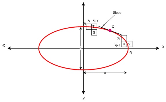
From point (0, b) to (a, 0), we can make their two parts based on the slope. At point Q, where the slope is -1.
The slope can be defined by f(x, y) = 0 = - (fx / fy) where fx and fy are partial derivatives of f(x, y) with respect to x and y.
$$\mathrm{f(x, y) \:=\: b^2x^2 \:+\: a^2y^2 \:-\: a^2b^2}$$
$$\mathrm{f_x \:=\: 2b^2x}$$
$$\mathrm{f_y \:=\: 2a^2y}$$
$$\mathrm{\frac{dy}{dx} \:=\: - \frac{2b^2x}{2a^2y}}$$
From this we can scan the slope to detect Q. We will start from (0, b).
Now consider the coordinates of the last pixel at step i is (xi, yi). We are to select either T (xi+1, yi) or S (xi+1, yi-1) will be the next pixel. So, the midpoint of T and S is needed for further decision making.
$$\mathrm{p_i \:=\: (f(x_{i\:+\:1}),\: y_i \:-\: 0.5)}$$
$$\mathrm{p_i \:=\: b^2 (x_{i\:+\:1})^2 \:+\: a^2 (y_i \:-\: 0.5)^2 \:-\: a^2b^2}$$
Based on the value of pi we can choose T or S. Thus the next steps are being calculated.
Here is the complete algorithm −
Input: Semi-major axis (a), Semi-minor axis (b), Center of ellipse (h, k)

Step 1: Initialize starting points and decision parameter
    x = 0
    y = b
    p1 = (b2) - (a2 * b) + (a2) / 4       // Decision parameter for Region 1

Step 2: Region 1: (Slope > -1)
    While (2 * b2 * x) <= (2 * a2 * y)    // Loop until slope reaches -1
        Plot points at (x+h, y+k), (-x+h, y+k), (x+h, -y+k), (-x+h, -y+k)

        If p1 < 0    // Midpoint is inside the ellipse
            p1 = p1 + (2 * b2 * (x + 1))
        Else         // Midpoint is outside or on the ellipse
            p1 = p1 + (2 * b2 * (x + 1)) - (2 * a2 * (y - 1))
            y = y - 1
        End If

        x = x + 1
    End While
Step 3: Initialize decision parameter for Region 2
    // Decision parameter for Region 2
    p2 = (b2 * (x + 0.5)2) + (a2 * (y - 1)2) - (a2 * b2)

Step 4: Region 2: (Slope <= -1)
    While y >= 0       // Loop until y reaches 0
        Plot points at (x+h, y+k), (-x+h, y+k), (x+h, -y+k), (-x+h, -y+k)

        If p2 > 0      // Midpoint is outside the ellipse
            p2 = p2 - (2 * a2 * (y - 1))
        Else           // Midpoint is inside the ellipse
            p2 = p2 - (2 * a2 * (y - 1)) + (2 * b2 * (x + 1))
            x = x + 1
        End If

        y = y - 1
    End While

Step 5: End
Example of the Midpoint Ellipse Algorithm
In this example, we take the centre coordinate at (0, 0), the major axis is 6 and the minor axis is 4.
| Iteration | x | y | Decision Parameter (p1/p2) | Points Generated |
|---|---|---|---|---|
| Start | 0 | 4 | Initial p1 = -119 | (0, 4), (0, -4) |
| 1 | 1 | 4 | p1 = -71 | (1, 4), (-1, 4), (1, -4), (-1, -4) |
| 2 | 2 | 4 | p1 = 9 | (2, 4), (-2, 4), (2, -4), (-2, -4) |
| 3 | 3 | 3 | p1 = -111 | (3, 3), (-3, 3), (3, -3), (-3, -3) |
| 4 | 4 | 3 | p1 = 33 | (4, 3), (-4, 3), (4, -3), (-4, -3) |
| 5 | 5 | 2 | p2 = -56 | (5, 2), (-5, 2), (5, -2), (-5, -2) |
| 6 | 6 | 1 | p2 = -320 | (6, 1), (-6, 1), (6, -1), (-6, -1) |
| 7 | 7 | 0 | p2 = -544 | (7, 0), (-7, 0), (7, 0), (-7, 0) |
Conclusion
In this chapter, we explained the concept of midpoint ellipse algorithm. This is an efficient technique for drawing ellipses in computer graphics. We understood how the algorithm works with the symmetry. Here, we were breaking the ellipse into regions, and using decision parameters to choose the best pixels to represent the curve. We also had a detailed example, showing the step-by-step implementation of the algorithm.