Cohen-Sutherland Line Clipping in Computer Graphics

---

---

Line clipping algorithm is used to remove the parts of lines that are outside the area viewport. Line clipping reduces the computation cost by enabling or disabling rendering operations within a defined region.

In this chapter, we will focus on one of the most frequently usedd line clipping algorithms in computer graphics: the Cohen-Sutherland Line Clipping Algorithm. We will go over the algorithm's basics, how it works, and cover an example for a better understanding.

Why Line Clipping is Needed?

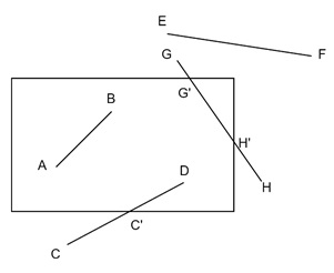
If we draw lines, they may be in any position. For example, there are four-line segments. AB, CD, EF and GH. The rectangle box is the viewport. Now if we see the lines, the line AB is inside the viewport completely. The EF is completely outside, so we can ignore EF. But for CD and GH we need special care. The C’D (part of CD) is inside the viewport, and (G’H’) part of GH is inside the viewport.

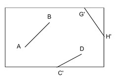
After clipping, it will be look like −

What is Cohen-Sutherland Line Clipping?

The Cohen-Sutherland Line Clipping Algorithm is used to determine which parts of a line segment lie inside a defined rectangular clipping window and which parts lie outside. The algorithm divides the 2D space into 9 regions. The middle region represents the area inside the clipping window, and the surrounding 8 regions represent the space outside.

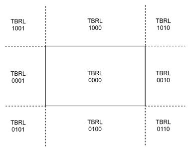
By using a simple 4-bit region code (TBRL), the algorithm can efficiently determine whether a line lies entirely inside, entirely outside, or partially inside the clipping window.

How the 4-Bit Region Code Works?

The 4-bit region code is used to identify the position of a point relative to the clipping window. Each bit in the code represents a direction (Top, Bottom, Right, Left). Here is how the code works:

• T (Top) − 1 if the point is above the window, 0 otherwise.
• B (Bottom) − 1 if the point is below the window, 0 otherwise.
• R (Right) − 1 if the point is to the right of the window, 0 otherwise.
• L (Left) − 1 if the point is to the left of the window, 0 otherwise.

Understanding the Nine Regions

The 9 regions in the Cohen-Sutherland algorithm represent:

• The center (the clipping window itself).
• The four corners (outside the window but diagonally).
• The four sides (top, bottom, left, and right).

Any point can be in one of these regions, and based on its location, the algorithm decides whether to display or clip the line.

How the Cohen-Sutherland Line Clipping Algorithm Works?

The Cohen-Sutherland Line Clipping Algorithm follows a step-by-step procedure to determine whether a line is fully inside, fully outside, or partially inside the clipping window. Here’s the process:

• Assign Region Codes − First, we calculate the region codes for both endpoints of the line. If both points have a region code of 0000, the line lies entirely inside the clipping window and is drawn without any further processing.
• Check for Trivial Rejection − If the bitwise AND of the region codes of the two points is not equal to 0000, the line is entirely outside the window and is discarded.
• Check for Partial Visibility − If one of the endpoints has a region code of 0000 but the other does not, or if both endpoints have non-zero region codes, the line is partially inside the window. In this case, the algorithm calculates the intersection points with the clipping boundaries and adjusts the line to fit within the window.
• Repeat as Necessary − If a line is partially inside the window, the process repeats for the shortened line segments until all parts of the line are either inside or discarded.

Example of Cohen-Sutherland Line Clipping

Let us go through an example to see how the Cohen-Sutherland Line Clipping Algorithm works in practice.

Problem

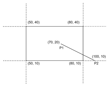
We are given a line with endpoints P1(70, 20) and P2(100, 10), and we need to clip this line against a clipping window with the following boundaries:

• Lower-left corner (50, 10)
• Upper-right corner (80, 40)

Step 1: Assign Region Codes

First, we calculate the region codes for P1 and P2.

For P1(70, 20) −

• xw_min = 50, xw_max = 80
• yw_min = 10, yw_max = 40

Since 50 ≤ 70 ≤ 80 and 10 ≤ 20 ≤ 40, the point P1 lies inside the window, so its region code is 0000.

For P2(100, 10): x = 100, which is greater than xw_max = 80. The y-coordinate is on the boundary yw_min = 10.

Therefore, the region code for P2 is 0010 (indicating that it is to the right of the window).

Step 2: Check for Trivial Cases

Since the region code of P1 is 0000 and the region code of P2 is 0010, the line is partially inside the window. We now need to find the intersection point where the line crosses the window boundary.

Step 3: Calculate the Intersection Point

The slope of the line P1P2 is calculated as −

• Slope (m) = (y2 - y1) / (x2 - x1)
• Slope (m) = (10 - 20) / (100 - 70) = -10 / 30 = -1/3

Next, we find the intersection point on the right boundary (x = 80). The equation of the line is −

• y - y1 = m(x - x1)
• y - 20 = (-1/3)(80 - 70)
• y - 20 = (-1/3) * 10
• y = 20 - 10/3 = 20 - 3.33 = 16.67

Thus, the intersection point is M(80, 16.67).

Step 4: Draw the Clipped Line

The visible portion of the line is between P1(70, 20) and the intersection point M(80, 16.67). The portion of the line beyond M is outside the window and is discarded.

So in this example, we clipped the line P1(70, 20) and P2(100, 10) against a window with boundaries (50, 10) and (80, 40). We calculated the intersection point on the right boundary and determined the visible portion of the line that lies within the clipping window.

Conclusion

In this chapter, we covered the basic principles of clipping, how the 4-bit region codes work, and how to determine whether a line is fully inside, fully outside, or partially inside a clipping window. We also walked through an example to understand the steps involved in calculating intersection points and determining the visible portion of a line.