Cyrus-Beck Line Clipping Algorithm in Computer Graphics

---

---

In this chapter, we will cover another line clipping algorithm which is known as the Cyrus-Beck Line Clipping Algorithm. We will explain how it works and see a detailed example. Also, we will highlight how this algorithm is different from other line clipping algorithms. We will cover the mathematics behind the algorithm and explore how it uses parametric line representation and dot products for clipping for a better understanding.

Cyrus-Beck Line Clipping Algorithm

The Cyrus-Beck Line Clipping Algorithm is a parametric line clipping method. It can use line clipping against a convex polygon window. This is new as compared to Cohen-Sutherland. This algorithm is more efficient than the Cohen-Sutherland Line Clipping Algorithm because it uses parametric equations and simpler calculations, like dot products, which make the process quicker and less complex.

Parametric Representation of a Line

In the Cyrus-Beck algorithm, a line is represented using a parametric equation. Suppose we have a line segment with endpoints P0 and P1. The parametric representation of this line is given by −

$$\mathrm{P(t) \:=\: P_0 \:+\: t\: \times\: (P_1 \:-\: P_0)}$$

Here −

• P0 is the starting point of the line.
• P1 is the ending point of the line.
• t is the parameter that varies between 0 and 1 to represent different points on the line.
• t = 0 represents the point P0.
• t = 1 represents the point P1.

The value of t helps in calculating intersection points which portions of the line are inside the clipping window.

How Does Cyrus-Beck Algorithm Work?

The Cyrus-Beck algorithm clips a line by checking whether the intersections of the line with the edges of the clipping window or not. We use dot product between the normal vector to the edge and the distance vector from a point on the edge to a point on the line. Depending on the value of this dot product, we can determine whether the point is inside, outside, or on the boundary of the window. Let us see the concepts in a concise way.

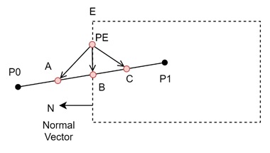
• Normal Vector (N) − For each edge of the window, we define a normal vector (N) that is perpendicular to the edge. This normal vector helps in determining the relative position of points on the line with respect to the edge.
• Distance Vector (P(t) - PE) − The distance vector is the vector from a point on the edge of the window (PE) to a point on the line (P(t)).
• Dot Product − The algorithm calculates the dot product between the normal vector and the distance vector. The value of the dot product tells us whether a point is inside, outside, or on the boundary of the window.

Conditions for Line Clipping

The Cyrus-Beck algorithm checks three conditions based on the value of the dot product:

• Dot Product > 0 − The point is outside the clipping window. In this case, the portion of the line that lies outside is discarded.
• Dot Product < 0 − The point is inside the clipping window. The portion of the line that lies inside the window is retained.
• Dot Product = 0 − The point lies on the boundary of the window. This means the line touches the window but does not lie entirely inside or outside.

Relation with Normal Vector

To calculate the intersection points between the line and the edges of the window, we need to follow the equation with normal N.

$$\mathrm{\mathbf{N} \:\cdot\: (P(t) \:-\: P_E)}$$

Which is nothing but −

$$\mathrm{| \mathbf{N} |\: \cdot\: | P(t) \:-\: P_E | \:\cos\: \theta}$$

For the above figure, for point B, the θ = 90°. So the dot product will be 0. And this signifies B is on the boundary.

For C the angle θ > 90°. So dot product is < 0 and C is inside the boundary.

Similarly for A, angle θ < 90°, dot product is > 0 and A is outside the boundary.

From this it is easily understandable which part should be clipped.

Finding the value of t

The value of t lies between 0 and 1, which represents points on the line between P0 and P1. If t lies within this range, the intersection point is valid.

To get the intersection point, as we know, N ⋅ (P(t) − PE) = 0. Which is nothing but

$$\mathrm{\mathbf{N}\: \cdot\: \left[ P_0 \:+\: t\: \times \:(P_1 \:-\: P_0) \:-\: P_E \right] \:=\: 0}$$

$$\mathrm{\text{i.e.,} \quad \mathbf{N}\: \cdot\: (P_0 \:-\: P_E) \:+\: \mathbf{N} \:\cdot \:t \left[ P_1 \:-\: P_0 \right] \:=\: 0}$$

Assume P1 P0 = D.

$$\mathrm{\mathbf{N} \:\cdot\: (P_0 \:-\: P_E) \:+\: \mathbf{N}\: \cdot \:t \:\cdot\: \mathbf{D} \:=\: 0}$$

$$\mathrm{- \mathbf{N}\: \cdot \:t \:\cdot\: \mathbf{D} \:=\: \mathbf{N} \:\cdot\: (P_0 \:-\: P_E)}$$

$$\mathrm{t \:=\: \frac{\mathbf{N} \:\cdot\: (P_0 \:-\: P_E)}{-\mathbf{N}\: \cdot\: \mathbf{D}}}$$

Conditions for Validity of t

For the Cyrus-Beck algorithm to work correctly, the following conditions must be satisfied:

• n ≠ 0 − The normal vector must not be zero.
• D ≠ 0 − The direction vector of the line should not be zero. If D = 0, it means P0 = P1, and the line is reduced to a single point, which is not valid for line clipping.
• n · D ≠ 0 − The line should not be parallel to the edge of the window. If the line is parallel, it either lies entirely inside or entirely outside the window, and no clipping is required.

Example of Cyrus-Beck Line Clipping

Let us go through an example to understand the process of line clipping using the Cyrus-Beck algorithm.

Problem

We are given a line segment with endpoints P0(70, 20) and P1(100, 10). The clipping window is a rectangle with boundaries −

• xw_min = 50, xw_max = 80
• yw_min = 10, yw_max = 40

We need to clip the line against this rectangular window using the Cyrus-Beck algorithm.

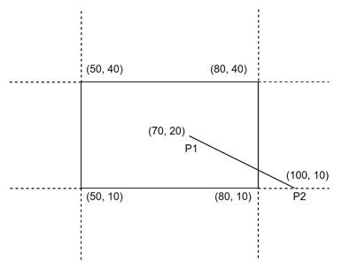
Step 1: Parametric Equation of the Line

The parametric equation of the line is −

$$\mathrm{P(t) \:=\: P_0 \:+\: t \:\times \:(P_1 \:-\: P_0)}$$

Substitute the coordinates of P0 and P1 −

$$\mathrm{P(t) \:=\: (70,\: 20) \:+\: t \:\times \:\left( (100, \:10) \:-\: (70,\: 20) \right)}$$

$$\mathrm{P(t) \:=\: (70,\: 20) \:+\: t \:\times\: (30, \:-10)}$$

$$\mathrm{P(t) \:= \:(70 \:+\: 30t,\: 20 \:-\: 10t)}$$

Step 2: Calculate the Normal Vectors for the Edges

Next, we calculate the normal vectors for each edge of the rectangular window. For example −

• For the left edge x = x_min, the normal vector is (-1, 0).
• For the right edge x = x_max, the normal vector is (1, 0).
• For the bottom edge y = y_min, the normal vector is (0, -1).
• For the top edge y = y_max, the normal vector is (0, 1).

Step 3: Calculate Intersection Points

We use the formula for t to calculate the intersection points.

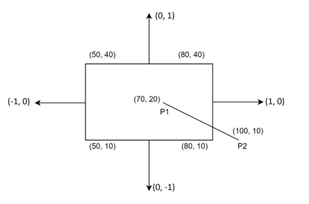
Let’s consider the intersection with the right edge x = 80 &mius;

$$\mathrm{t \:=\: \frac{N \:\cdot\: (P_0 \:-\: P_E)}{-N\: \cdot\: D}}$$

Where:

• N = (1, 0) (normal vector for the right edge).
• P0 = (70, 20).
• Pe = (80, 10) (a point on the right edge).
• D = (30, -10) (direction vector of the line).

Calculate t and find the intersection points. Repeat this process for other edges to determine the visible portion of the line.

Conclusion

In this chapter, we explained the Cyrus-Beck Line Clipping Algorithm in computer graphics. We covered the basics of the algorithm, including how it uses parametric line representation and dot products to perform line clipping. We also walked through an example to illustrate the process of calculating the intersection points and clipping a line.