Computing Viewing Rays in Ray Tracing

---

---

Viewing Rays help to determine which objects in a 3D scene are visible from the cameras perspective and which objects are not visible. Each viewing ray starts from a specific point and travels in a particular direction. It can be used to trace the path of light through the scene and produce realistic images.

Read this chapter to understand the process of computing viewing rays in ray tracing and learn the different methods used in this process.

What are Viewing Rays?

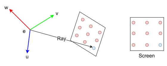
Viewing rays define how the camera views the objects in a scene. Each viewing ray starts from a point in the cameras view and travels through the scene to determine which objects are visible. When a viewing ray intersects an object, it is used to calculate the color and shading of the corresponding pixel on the image plane.

To generate viewing rays, we first need to define the camera geometry. This includes the cameras position (called the viewpoint), the image plane, and the direction in which the rays will travel. By adjusting these parameters, we can create different types of views, such as orthographic or perspective views.

Camera Frame and Ray Representation

We have seen a little of this concept in the last article, let us see them in detail. A viewing ray is represented mathematically as a parametric line. It has an origin point and a direction vector. In ray tracing, the ray can be defined using the formula −

$$\mathrm{p(t) \:=\: e \:+\: t(s \:-\: e)}$$

Where,

• p(t) is a point on the ray at distance t from the origin.
• e is the origin of the ray, usually the camera's viewpoint.
• s - e is the direction of the ray.
• t is a parameter that determines how far along the ray we want to go.

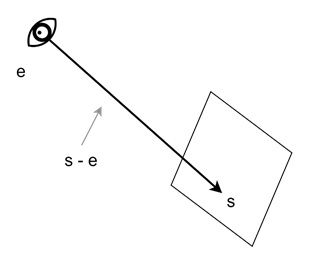
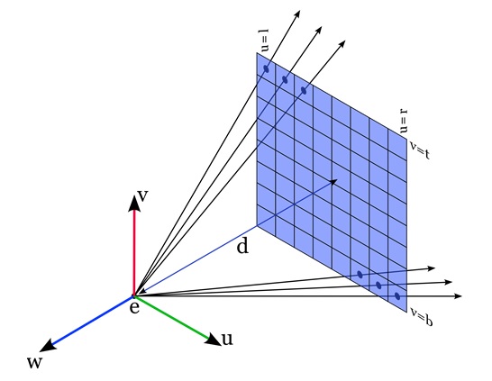
In the figure, the ray coming from the eye to a point on the image plane. This formula tells us that starting from e, we can move in the direction (s – e) to find any point along the ray. The point s represents a position on the image plane. The value of t controls how far we move along the direction vector (s – e).

• If t < 0, the point is behind the camera.
• If t > 1, the point is farther away from the camera than s.

Using the Camera Frame

To compute viewing rays, we need a reference frame called the camera frame. The camera frame is made up of three vectors: u, v, and w. These vectors define the cameras orientation and position in the 3D space. The camera frame is also centered at the cameras viewpoint, e.

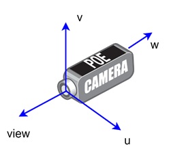
• u vector − Points to the right from the camera’s perspective.
• v vector − Points upward from the camera’s perspective.
• w vector − Points backward, opposite to the view direction.

The u, v, and w vectors form an orthonormal coordinate system. This means they are perpendicular to each other and have a unit length. The camera frame helps us define where the rays originate and in which direction they travel. −

Generating Rays for Orthographic Views

In an orthographic view, all the rays have the same direction but start at different positions on the image plane. Orthographic views are often used for technical and architectural drawings because they preserve the size and shape of objects.

To generate orthographic viewing rays, follow the steps given below −

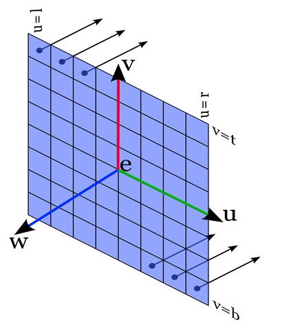
• We start from defining the image plane using four numbers, l, r, b, and t. These numbers represent the left, right, bottom, and top edges of the image.
• We then compute the position of each pixel on the image plane. The position of a pixel at (i, j) in the raster image can be calculated as:

$$\mathrm{u \:=\: l \:+\: (r \:-\: l) \:\cdot\: \frac{i \:+\: 0.5}{nx}}$$

$$\mathrm{v \:=\: b \:+\: (t \:-\: b) \:\cdot\: \frac{j \:+\: 0.5}{ny}}$$

Where:

• nx and ny are the number of pixels in the x and y directions.
• u and v are the coordinates of the pixel’s position on the image plane.

The direction of each ray is the same and equal to the view direction, -w.

The origin of each ray is calculated using the pixel’s position on the image plane and the camera’s origin.

In an orthographic view, rays do not converge. This means that objects farther away do not appear smaller, and parallel lines remain parallel in the final image.

Generating Rays for Perspective Views

In a perspective view, all the rays originate from the same viewpoint but travel in different directions. Perspective views make objects farther away appear smaller and give a realistic sense of depth.

To generate perspective viewing rays −

• We define the camera’s viewpoint, e, and the image plane. The image plane is positioned at a certain distance d in front of the viewpoint.
• For each pixel on the image plane, we compute the direction of the ray using the formula −

$$\mathrm{\text{ray direction} \:=\: \frac{s \:-\: e}{|s \:-\: e|}}$$

Where −

• s is the position of the pixel on the image plane.
• e is the viewpoint of the camera.
• |s - e| is the distance between s and e.
• The direction of each ray is different because s varies with the pixel's position.

Conclusion

In this chapter, we explained how to compute viewing rays in ray tracing. We also understood the concept of viewing rays and how they are represented using the camera frame.

We explained how to generate rays for both orthographic and perspective views. For orthographic views, all rays have the same direction but start at different positions. For perspective views, all rays start from the same viewpoint but travel in different directions.