Procedural 3D Textures for Texture Mapping

---

---

So far in this tutorial, we have covered several different concepts of texture mapping for 3D objects. We have learnt the traditional texture mapping usage of 2D images that are mapped onto 3D surfaces. However, when it comes to complex or irregular surfaces, this method can lead to distortions. A more flexible and efficient alternative is Procedural 3D textures. These textures are generated using mathematical functions and are defined at every point in 3D space.

In this chapter, we will explain what procedural 3D textures are and how they work. We will also highlight some common examples like 3D stripes, solid noise, and turbulence.

What are Procedural 3D Textures?

Procedural 3D textures define color and surface properties of a 3D object using a mathematical function, and not directly a 2D image. This function, usually denoted as cr(p), maps 3D points (p) to RGB colors.

Unlike traditional 2D textures, procedural 3D textures work in 3D space and are not constrained to the surface of an object. This method is particularly useful for objects that have a solid appearance, like marble sculptures or wood grains.

The main advantage of procedural 3D textures is that they avoid the complexities and limitations of mapping a 2D texture onto a 3D surface. Since the texture is already defined in 3D space, there is no need to worry about distortion. However, storing these textures as 3D raster images can consume a large amount of memory. Therefore, procedural textures are often generated using mathematical procedures, rather than storing them as precomputed images.

Creating 3D Procedural Textures

There are several basic methods to create 3D procedural textures. These methods use mathematical functions to generate the texture at any point in 3D space. The following sections discuss some of the most common techniques used to create procedural textures: 3D stripe textures, solid noise, and turbulence.

3D Stripe Textures

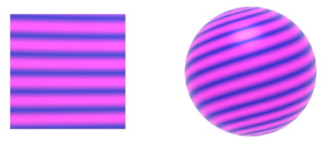
Let us see the stripe texture first. Creating a striped texture is a straightforward example of a 3D procedural texture. We can define a stripe texture using two colors, c0 and c1. The texture is generated using an oscillating function, such as a sine function, that alternates between these two colors.

Example

Here's a basic example of how to create a 3D stripe texture −

RGB stripe(point p) {
   if (sin(xp) > 0) {
      return c0;
   } else {
      return c1;
   }
}

This algorithm generates a simple stripe pattern that changes color based on the x-coordinate of the point p. We can also control the width of the stripes using a parameter w −

RGB stripe(point p, real w) {
   if (sin(xp / w) > 0) {
      return c0;
   } else {
      return c1;
   }
}

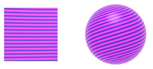
This parameter w determines the frequency of the sine wave, thereby changing the width of the stripes. To make the color transition between stripes smoother, we can introduce a blending parameter t −

RGB stripe(point p, real w) {
   t = (1 + sin(px / w)) / 2;
   return (1  t) * c0 + t * c1;
}

Using these functions, we can create various types of stripe textures, from hard-edged stripes to smoothly blended ones. Figure 11.26 in the source material shows different stripe textures created using these techniques.

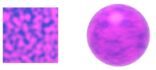
Solid Noise

Stripe textures are present in many natural textures. Sometimes, we need much more random textures, like the speckled patterns on birds’ eggs, require more randomness. To achieve this, we use solid noise. These are sometimes referred to as Perlin noise.

Perlin noise is a type of noise function that generates smooth, continuous random values across 3D space. It is named after its creator, Ken Perlin, who developed it to simulate natural textures in computer graphics.

Simply using random numbers for every point in space would result in a “white noise” effect, similar to TV static. This kind of randomness does not look natural because there is no correlation between nearby points. To create a smoother noise texture, Perlin used a technique that interpolates between random values at lattice points.

The basic steps to generate Perlin noise are −

• Create a lattice with random values at each point.
• Use Hermite interpolation to ensure smooth transitions between points.
• Use random vectors rather than random values. This helps reduce the grid-like appearance.

Perlin noise is computed using the formula −

$$\mathrm{n \:=\: (x,\: y,\: z) \:=\: \sum_{i = \lfloor x \rfloor}^{\lfloor x \rfloor + 1}\: \sum_{j = \lfloor y \rfloor}^{\lfloor y \rfloor + 1}\: \sum_{k = \lfloor z \rfloor}^{\lfloor z \rfloor + 1}\: \Omega_{ijk} (x \:-\: i,\: y \:-\: j,\: z \:-\: k)}$$

Where (x, y, z) are cartesian coordinate of x, and

$$\mathrm{\Omega_{ijk}(u,\: v,\: w) \:=\: \omega(u) \omega(v) \omega(w) \left( \Gamma_{ijk}(u,\: v,\: w) \right)}$$

ω(t) is a cubic weighting function and Γ_ijk is a random unit vector at each lattice point (i, j, k). Perlin noise can be used to create a wide range of textures, such as clouds, marble, or wood grain.

Turbulence Texture

Turbulence texture is a common technique used in procedural texturing. It just adds multiple layers of noise at different scales to create a texture with features of varying sizes. This gives the texture a more complex and natural appearance.

The turbulence function is defined as −

$$\mathrm{n_t(x) \:=\: \sum_i \:\frac{|n(2^i x)|}{2^i}}$$

In this function, each term in the summation adds a layer of noise at a different scale. The absolute value shows that each layer contributes only positive values, creating a coherent texture. Turbulence can be used to create textures like water, smoke, or clouds.

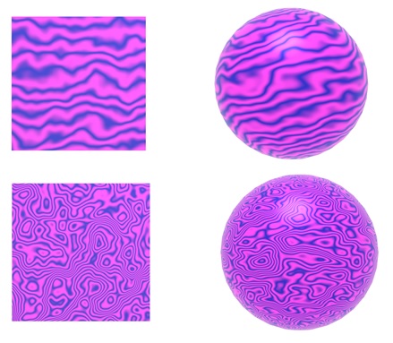
Turbulence can also be combined with other textures. For example, it can be used to distort a stripe texture −

RGB turbstripe(point p, double w) {
   double t = (1 + sin(k1 * zp + turbulence(k2 * p)) / w) / 2;
   return t * s0 + (1 - t) * s1;
}

By adjusting the parameters k1 and k2, we can create a variety of effects. Figure 11.30 in the source material shows different turbulent stripe textures generated using this function.

Benefits of Procedural 3D Textures

In the procedural 3D textures, they offer several benefits over traditional 2D textures:

• No Distortion − Since the texture is defined in 3D space, there is no distortion when it is applied to complex surfaces.
• Infinite Detail − Procedural textures can be generated at any level of detail, making them suitable for zooming in without losing quality.
• Memory Efficiency − Procedural textures are defined mathematically, so they don’t require large amounts of memory to store image data.
• Flexibility − A wide range of textures can be created using the same basic functions, offering more flexibility compared to precomputed textures.

Conclusion

In this chapter, we explained the basic concept of procedural 3D textures for texture mapping in computer graphics. We started by explaining what procedural 3D textures are and how they differ from traditional 2D textures. We then discussed different methods to create procedural textures, including 3D stripe textures, solid noise, and turbulence.

Finally, we understood the benefits of using procedural textures. Procedural 3D textures are powerful tools for adding rich, detailed textures to complex surfaces in computer graphics.