Mid-point Circle Generation Algorithm

---

---

The Mid-point Circle Generation Algorithm works by determining the points needed for rasterizing it. It is efficient because it calculates the points present in the first octant of the circle and uses the circle's symmetry to generate the remaining points for the other seven octants.

In this chapter, we will explain the basics of the mid-point circle generation algorithm and go through a detailed example. We will also cover its step-by-step implementation for a better understanding.

Basics of Mid-Point Circle Generation Algorithm

The main idea of the Mid-point Circle Generation Algorithm is to determine whether a pixel lies inside, on, or outside the boundary of a circle. We plot the points for one-eighth of the circle (the first octant) and use the symmetry of the circle to replicate those points in the other octants.

Symmetry of Circles

As we have seen in the last algorithm also the circle generation has been done with the idea of symmetry. We generate for only 45 and rest can be easily calculated with changing the coordinate values, since a circle is symmetric about its center.

For a circle with a center at (0,0) and radius r, the equation of the circle is −

$$\mathrm{x^2 \:+\: y^2 \:=\: r^2}$$

Given a point P(x, y) on the circle, the decision to plot the next point depends on whether the midpoint between two possible pixels lies inside or outside the circle.

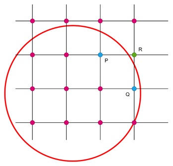
Here, P and Q both points are inside the circle, whereas the point R is outside of the circle.

The Algorithm

The algorithm follows these steps −

• Start with an initial point − The first point to be plotted is (r, 0), which lies on the positive X-axis.
• Calculate the initial decision parameter − The initial decision parameter is computed as −

$$\mathrm{P_1 \:=\: 1 \:-\: r}$$

• Iterate through points in the first octant − For each subsequent point, we check whether the next pixel is above or below the circle or not. The next pixel is either at $\mathrm{(x,\: y \:+\: 1) \text{ or } (x \:-\: 1,\: y \:+\: 1)}$
  • If the decision parameter is less than or equal to zero, the midpoint is inside the circle. In this case, the next pixel is $\mathrm{(x,\: y\: +\: 1)}$.
  • If the decision parameter is greater than zero, the midpoint is outside the circle. The next pixel is $(x - 1, y + 1)$.
• Update the decision parameter − For each new pixel, update the decision parameter depending on which pixel was chosen.
  • If the midpoint was inside or on the circle −

  $$\mathrm{P_{k+1} \:=\: P_k \:+\: 2y_k \:+\: 1}$$

  • If the midpoint was outside the circle −

  $$\mathrm{P_{k+1} \:=\: P_k \:+\: 2y_k \:-\: 2x_k \:+\: 1}$$

Example of Mid-Point Circle Generation

Let us go through a detailed example where we apply the Mid-point Circle Generation Algorithm.

Consider the center is at location (0,0), and Radius is 3.

Let's understand the step-by-step calculation.

Starting point − The first point to plot is (3, 0) on the x-axis.

Initial decision parameter − Using the formula, the initial decision parameter P₁ is −

$$\mathrm{P_1 \:=\: 1 \:-\: r \:=\: 1 \:-\: 3 \:=\: -2}$$

First iteration − For the first iteration, we start with x = 3 and y = 0. Since P₁ = − 2 (which is less than 0), the next point is (3, 1). The new decision parameter is −

$$\mathrm{P_2 \:=\: P_1 \:+\: 2y_1 \:+\: 1 \:=\: -2 \:+\: 2(0) \:+\: 1}$$

The points at this stage are: (3, 0), (−3, 0), (0, 3), and (0, −3). Using symmetry, we also plot (3, 1), (−3, 1), (3, −1), and (−3, −1).

Second iteration − For the second iteration, with x = 3 and y = 1, since P₂ = −1 (which is less than 0), the next point is (3, 2). The new decision parameter is −

$$\mathrm{P_3 \:=\: P_2 \:+\: 2y_2 \:+\: 1 \:=\: -1 \:+\: 2(1) \:+\: 1 \:=\: 2}$$

The points at this stage are: (3, 2), (3,2), (3, 2), and (3, 2)

Third iteration − Now, for the third iteration, with x = 3 and y = 2 since P₃ = 2 (which is greater than 0), the next point is (2, 3). The new decision parameter is −

$$\mathrm{P_4 \:=\: P_3 \:+\: 2y_3 \:-\: 2x_3 \:+\: 1 \:=\: 2 \:+\: 2(2) \:-\: 2(3) \:+\: 1 \:=\: 3}$$

The points at this stage are: (2, 3), (2, 3), (2, 3), and (2, 3)

Final iteration − For the final iteration, with x = 2 and y = 3, since P₄ = 3 (which is greater than 0), the next point is (1, 3). The decision parameter is updated, but since x is now smaller than y, the algorithm stops.

The points at this stage are: (1, 3), (1, 3), (1, 3), and (1,3)

Full Set of Points − After completing all iterations, we have the following points for the circle with a radius of 3 and center at (0,0) −

(3, 0), (3, 0), (0, 3), (0, 3), (3, 1), (3, 1), (3, 1), (3, 1), (3, 2), (3, 2), (3, 2), (3, 2), (2, 3), (2, 3), (2, 3), (2, 3), (1, 3), (1, 3), (1, 3), (1, 3).

Conclusion

In this chapter, we explained the Mid-point circle generation algorithm in detail. We started the chapter with a brief discussion on the symmetry of circles, which forms the basis of the algorithm. Then, we outlined the steps of the algorithm, explaining how the decision parameter helps in determining the next point to plot. Finally, we worked through an example with a radius of 3 to explain the algorithm in action.