- Computer Graphics - Home
- Computer Graphics Basics
- Computer Graphics Applications
- Graphics APIs and Pipelines
- Computer Graphics Maths
- Sets and Mapping
- Solving Quadratic Equations
- Computer Graphics Trigonometry
- Computer Graphics Vectors
- Linear Interpolation
- Computer Graphics Devices
- Cathode Ray Tube
- Raster Scan Display
- Random Scan Device
- Phosphorescence Color CRT
- Flat Panel Displays
- 3D Viewing Devices
- Images Pixels and Geometry
- Color Models
- Line Generation
- Line Generation Algorithm
- DDA Algorithm
- Bresenham's Line Generation Algorithm
- Mid-point Line Generation Algorithm
- Circle Generation
- Circle Generation Algorithm
- Bresenham's Circle Generation Algorithm
- Mid-point Circle Generation Algorithm
- Ellipse Generation Algorithm
- Polygon Filling
- Polygon Filling Algorithm
- Scan Line Algorithm
- Flood Filling Algorithm
- Boundary Fill Algorithm
- 4 and 8 Connected Polygon
- Inside Outside Test
- 2D Transformation
- 2D Transformation
- Transformation Between Coordinate System
- Affine Transformation
- Raster Methods Transformation
- 2D Viewing
- Viewing Pipeline and Reference Frame
- Window Viewport Coordinate Transformation
- Viewing & Clipping
- Point Clipping Algorithm
- Cohen-Sutherland Line Clipping
- Cyrus-Beck Line Clipping Algorithm
- Polygon Clipping Sutherland–Hodgman Algorithm
- Text Clipping
- Clipping Techniques
- Bitmap Graphics
- 3D Viewing Transformation
- 3D Computer Graphics
- Parallel Projection
- Orthographic Projection
- Oblique Projection
- Perspective Projection
- 3D Transformation
- Rotation with Quaternions
- Modelling and Coordinate Systems
- Back-face Culling
- Lighting in 3D Graphics
- Shadowing in 3D Graphics
- 3D Object Representation
- Represnting Polygons
- Computer Graphics Surfaces
- Visible Surface Detection
- 3D Objects Representation
- Computer Graphics Curves
- Computer Graphics Curves
- Types of Curves
- Bezier Curves and Surfaces
- B-Spline Curves and Surfaces
- Data Structures For Graphics
- Triangle Meshes
- Scene Graphs
- Spatial Data Structure
- Binary Space Partitioning
- Tiling Multidimensional Arrays
- Color Theory
- Colorimetry
- Chromatic Adaptation
- Color Appearance
- Antialiasing
- Ray Tracing
- Ray Tracing Algorithm
- Perspective Ray Tracing
- Computing Viewing Rays
- Ray-Object Intersection
- Shading in Ray Tracing
- Transparency and Refraction
- Constructive Solid Geometry
- Texture Mapping
- Texture Values
- Texture Coordinate Function
- Antialiasing Texture Lookups
- Procedural 3D Textures
- Reflection Models
- Real-World Materials
- Implementing Reflection Models
- Specular Reflection Models
- Smooth-Layered Model
- Rough-Layered Model
- Surface Shading
- Diffuse Shading
- Phong Shading
- Artistic Shading
- Computer Animation
- Computer Animation
- Keyframe Animation
- Morphing Animation
- Motion Path Animation
- Deformation Animation
- Character Animation
- Physics-Based Animation
- Procedural Animation Techniques
- Computer Graphics Fractals
Physics-Based Animation in Computer Graphics
Physics-based animations are the technique used in computer graphics to simulate real-world physical laws and apply them to animated objects. These laws show how objects behave when subjected to forces like gravity, collisions, and other environmental factors.
Physics-based animation is often used when traditional animation techniques are insufficient to create realistic effects. This is when the elements are like fluids, cloth, and rigid bodies, etc.
In this chapter, we will see the fundamentals of physics-based animation, the key techniques involved, and their applications in creating realistic motion in animation. We will also see the challenges of using this method for a better understanding.
Basics of Physics-Based Animation
Physics-based animations require differential equations that describe physical phenomena. These equations are the mathematical representation of physical laws. To solve differential equations, animators need to simulate real-world behavior. For example, to animate an object falling under the force of gravity, an equation representing the force of gravity is solved over time to compute the object's position and speed.
There are two main types of differential equations: ordinary differential equations (ODEs) and partial differential equations (PDEs). ODEs work with functions of a single variable, while PDEs deal with functions of multiple variables such as time and space. The complexity of these equations means that solving them analytically is often difficult or impossible. Instead, numerical methods are used to approximate the solutions.
Applications of Physics-Based Animation
Physics-based animation is particularly useful in situations where other animation techniques, do not produce realistic results. Some of the most common applications include −
- Fluid Animation − Fluids, including water, smoke, clouds, and fire, are difficult to animate using traditional techniques. Physics-based animation allows for realistic simulations of fluid dynamics.
- Cloth Simulation − Simulating the movement of cloth in response to forces like wind, gravity, and collisions requires accurate modelling of how the fabric behaves. Figure 16.22 provides an example of realistic cloth simulation.
- Rigid Body Motion − The movement of solid objects like cars or rocks can be accurately simulated using physics-based techniques.
- Elastic Object Deformation − Elastic materials, such as rubber, can be deformed in response to forces. Physics-based animation ensures that the deformation is realistic and smooth.
Let us see some of the examples for a clear understanding. At first, we will see the explosion effect.
The following example demonstrates fluid animation −
The following example shows cloth animation −
Finite Difference Method
Let us enter into a little maths on physics based animations. One of the most common techniques used in physics-based animation is the finite difference method. This method is conceptually simple and has been applied to a wide range of problems in animation. The idea behind this method is to replace the differential equations governing physical motion with difference equations.
The process shows breaking down a continuous domain, such as time or space, into a finite number of points. These points form a grid, and the values of the unknown function (such as position or velocity) are calculated at each point. The derivatives in the original equation are then approximated using the values at nearby grid points.
For example, the derivative of a function f(t) with respect to time can be approximated using the following equation −
$$\mathrm{\frac{df(t)}{dt} \:\approx\: \frac{\Delta f}{\Delta t} \:=\: \frac{f(t \:+\: \Delta t) \:-\: f(t)}{\Delta t}}$$
By repeatedly solving these difference equations, the animator can propagate the solution forward in time, simulating the motion of the object.
Explicit and Implicit Schemes
There are two primary ways to compute the values of a function at future time steps: explicit schemes and implicit schemes.
Explicit Schemes
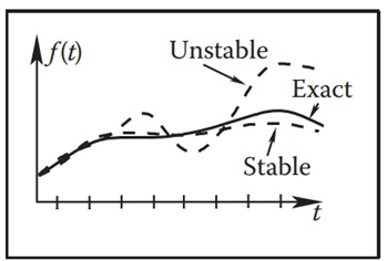
In an explicit system, the value of the unknown function at the next time step f(t + Δt) is calculated using only the known values from the current time step. This makes explicit schemes simple and efficient to implement. However, they can be unstable.
An unstable scheme can cause the solution to deviate significantly from the true behavior of the system, as shown in the following figure.
Implicit Schemes
In an implicit system, the function values at future time steps are mixed with the values from the current time step. This is requiring the solution of a system of equations. Although implicit schemes are more computationally expensive, they are generally more stable, allowing for larger time steps without sacrificing accuracy.
Implicit schemes are often used when stability is critical, such as in simulations involving collisions or fast-moving objects.
Challenges in Physics-Based Animation
Physics based animations are simulated and may not be accurate with real sense. Though let us see their challenges at once. One of the main difficulties is the complexity of the underlying mathematical models. Animators need a good understanding of physics and numerical methods to set up and solve the equations correctly.
Another challenge is computational cost. Physics-based animation is often more resource-intensive than other techniques, requiring significant processing power and time to simulate large or complex systems, such as a fluid simulation or a scene with many interacting objects.
One of the most difficult problems in physics-based animation is collision detection. When objects collide, their motion changes abruptly. Detecting and resolving these collisions requires solving complex geometric problems, which can slow down the simulation. As such, efficient collision detection algorithms are crucial for creating realistic and timely results.
Controlling Physics-Based Animation
One of the key limitations of physics-based animation is that it can be difficult to control the outcome. The motion is determined by the physical laws and initial conditions, leaving the animator with little direct control over the behavior of the objects. If the result does not meet the animator's expectations, they have limited options for making adjustments.
The animator can modify the initial conditions, adjust the physical properties of the system (such as mass or elasticity), or add artificial terms to the equations to "drive" the solution in a specific direction. However, making these changes requires a deep understanding of both physics and numerical techniques. Without careful adjustments, the realism of the animation can be compromised.
Conclusion
In this chapter, we explained the concept of physics-based animation in computer graphics. We started by discussing the basics of how physical laws represented by differential equations. They are used to simulate realistic motion. We then understood applications of physics-based animation, such as fluid animation, cloth simulation, and rigid body motion etc.
We covered the finite difference method, which is one of the most popular techniques for solving differential equations. We also understood the challenges of physics-based animation, including its complexity, computational cost, and the difficulty of controlling the outcome.