Polygon Clipping Sutherland-Hodgman Algorithm

---

---

After understanding the concept of line clipping, let us now learn something more advanced. In this chapter, we will show how to clip some shape or a polygon. One of the most widely used algorithms for polygon clipping is the Sutherland-Hodgman Algorithm. This algorithm handles the clipping of polygons by processing each edge of the window individually.

In this chapter, we will cover the Sutherland-Hodgman Polygon Clipping Algorithm, explain how it works, and walk through a detailed example for a better understanding.

What is Polygon Clipping?

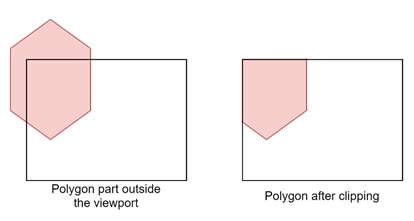
Polygon clipping is the process of removing certain parts of a polygon that fall outside a specified rectangular boundary. We call this the viewport. The aim is to display only the part of the polygon that is within the window. Any portion of the polygon that extends outside the window will be clipped off, ensuring that the polygon fits neatly inside the viewing area.

Sutherland-Hodgman Algorithm

The Sutherland-Hodgman Algorithm clips a polygon one edge at a time. The clipping process involves four stages:

• Left Clipping − Clipping the parts of the polygon that are outside the left edge of the window.
• Right Clipping − Clipping the parts of the polygon that are outside the right edge of the window.
• Top Clipping − Clipping the parts of the polygon that are outside the top edge of the window.
• Bottom Clipping − Clipping the parts of the polygon that are outside the bottom edge of the window.

The key characteristic of this algorithm is that the output of each clipping step becomes the input for the next step. This way, by the end of all four steps, any part of the polygon that lies outside the window will be removed.

How the Sutherland-Hodgman Algorithm Works?

The Sutherland-Hodgman Algorithm clips each polygon edge based on its relationship to the clipping window. It follows a set of rules to determine which parts of the polygon to keep and which parts to discard. The process can be broken down into four cases −

Case 1: Edge from Inside to Outside − If the edge of the polygon goes from inside the window to outside, the point where the edge exits the window is calculated. This point becomes part of the clipped polygon. The portion of the edge outside the window is discarded.

Case 2: Edge from Outside to Inside − If the edge goes from outside the window to inside, the point where the edge enters the window is calculated. Then both this point and the following vertex inside the window are kept. The portion outside is discarded.

Case 3: Edge Completely Inside − If the entire edge of the polygon lies inside the window, both vertices of the edge are retained.

Case 4: Edge Completely Outside − If the edge lies completely outside the window, it is discarded entirely.

These four cases allow the algorithm to process each edge of the polygon and determine whether it should be kept, clipped, or partially retained. This process is repeated for all four edges of the window (left, right, top, and bottom).

Steps of the Sutherland-Hodgman Algorithm

The Sutherland-Hodgman Algorithm works through a series of clipping operations. Each step uses the output from the previous step as its input. Let us break down the steps −

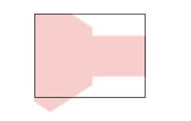
Consider the polygon and window on which we will apply clipping.

Step 1: Left Clipping

In the first step, the algorithm clips the polygon against the left edge of the window. Any part of the polygon that extends to the left of the window is clipped off. The output of this step is the clipped polygon, which is passed as input to the next step.

Step 2: Right Clipping

Next, the algorithm clips the polygon against the right edge of the window. The process is like the left clipping. This time it removes any parts of the polygon that lie outside the right boundary. The output is again passed to the next step.

Step 3: Top Clipping

In the third step, the algorithm performs top clipping. It removes the portions of the polygon that lie above the top boundary of the window. The resulting polygon is then passed to the final step.

Step 4: Bottom Clipping

Finally, the algorithm clips the polygon against the bottom edge of the window. Any parts of the polygon that extend below the bottom boundary are clipped. The final output is the clipped polygon, which now fits entirely within the window.

Example of Sutherland-Hodgman Polygon Clipping

Let us go through a numeric example to understand how the Sutherland-Hodgman Algorithm works.

Problem

We are given a rectangular window and a polygon (square) with vertices −

• V1(25, 30)
• V2(40, 45)
• V3(55, 30)
• V4(40, 15)

The clipping window is defined by −

$$\mathrm{x_{\text{min}} \:=\: 30,\: \quad x_{\text{max}} \:=\: 50}$$

$$\mathrm{y_{\text{min}} \:=\: 20,\: \quad y_{\text{max}} \:=\: 40}$$

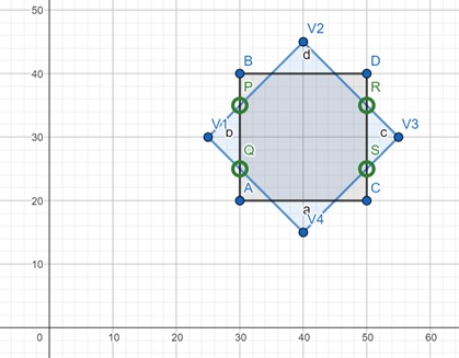
Showing the window as ABDC −

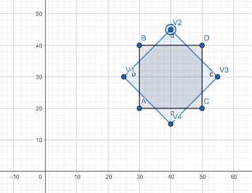
We need to clip the polygon using the Sutherland-Hodgman Algorithm.

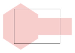
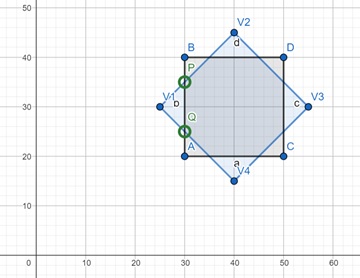
Step 1: Left Clipping

First, we perform clipping against the left boundary (x_min = 30). The polygon edges are:

V1(25, 30) to V2(40, 45): This edge crosses from left to inside, so we calculate the intersection point and update the edge as P(30, 35) to V2(40, 45).

V2(40, 45) to V3(55, 30): This edge at right of the left edge, so no clipping is needed.

V3(55, 30) to V4(40, 15): This edge at right of the left edge, so no clipping is needed.

V4(40, 15) to V1(25, 30): This edge crosses from inside to left, so we calculate the intersection point and update the edge as Q(30, 25) to P(30, 35).

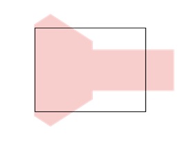
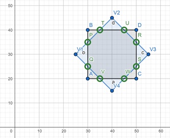
Step 2: Right Clipping

Next, we perform right clipping against x_max = 50:

V2(40, 45) to V3(55, 30) : Crosses right boundary, so we calculate the intersection point and update as V2(40, 45) to R(50, 35).

Then, clip V3 to V4, the intersection is S(50,25)

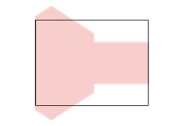
Step 3: Top Clipping

Now, we clip against the top boundary (y_max = 40) −

Here clipping are from P to V2 and V2 to R. The intersections are T(35, 40) and U(45, 40)

Step 4: Bottom Clipping

Finally, we clip against the bottom boundary (y_min = 20):

The bottom part contains segments Q to V4 and V4 to S, with intersections V(35, 20) and W(45, 20)

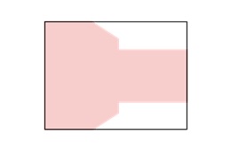
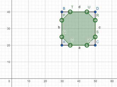
The final clipped polygon looks like this −

Conclusion

In this chapter, we explained the Sutherland-Hodgman Polygon Clipping Algorithm in computer graphics. We started by understanding the concept of polygon clipping and why it is important for rendering objects inside a window. We then discussed the four steps involved in the Sutherland-Hodgman Algorithm: left, right, top, and bottom clipping. Finally, we walked through a detailed example to demonstrate how the algorithm works in practice.