- Computer Graphics - Home
- Computer Graphics Basics
- Computer Graphics Applications
- Graphics APIs and Pipelines
- Computer Graphics Maths
- Sets and Mapping
- Solving Quadratic Equations
- Computer Graphics Trigonometry
- Computer Graphics Vectors
- Linear Interpolation
- Computer Graphics Devices
- Cathode Ray Tube
- Raster Scan Display
- Random Scan Device
- Phosphorescence Color CRT
- Flat Panel Displays
- 3D Viewing Devices
- Images Pixels and Geometry
- Color Models
- Line Generation
- Line Generation Algorithm
- DDA Algorithm
- Bresenham's Line Generation Algorithm
- Mid-point Line Generation Algorithm
- Circle Generation
- Circle Generation Algorithm
- Bresenham's Circle Generation Algorithm
- Mid-point Circle Generation Algorithm
- Ellipse Generation Algorithm
- Polygon Filling
- Polygon Filling Algorithm
- Scan Line Algorithm
- Flood Filling Algorithm
- Boundary Fill Algorithm
- 4 and 8 Connected Polygon
- Inside Outside Test
- 2D Transformation
- 2D Transformation
- Transformation Between Coordinate System
- Affine Transformation
- Raster Methods Transformation
- 2D Viewing
- Viewing Pipeline and Reference Frame
- Window Viewport Coordinate Transformation
- Viewing & Clipping
- Point Clipping Algorithm
- Cohen-Sutherland Line Clipping
- Cyrus-Beck Line Clipping Algorithm
- Polygon Clipping Sutherland–Hodgman Algorithm
- Text Clipping
- Clipping Techniques
- Bitmap Graphics
- 3D Viewing Transformation
- 3D Computer Graphics
- Parallel Projection
- Orthographic Projection
- Oblique Projection
- Perspective Projection
- 3D Transformation
- Rotation with Quaternions
- Modelling and Coordinate Systems
- Back-face Culling
- Lighting in 3D Graphics
- Shadowing in 3D Graphics
- 3D Object Representation
- Represnting Polygons
- Computer Graphics Surfaces
- Visible Surface Detection
- 3D Objects Representation
- Computer Graphics Curves
- Computer Graphics Curves
- Types of Curves
- Bezier Curves and Surfaces
- B-Spline Curves and Surfaces
- Data Structures For Graphics
- Triangle Meshes
- Scene Graphs
- Spatial Data Structure
- Binary Space Partitioning
- Tiling Multidimensional Arrays
- Color Theory
- Colorimetry
- Chromatic Adaptation
- Color Appearance
- Antialiasing
- Ray Tracing
- Ray Tracing Algorithm
- Perspective Ray Tracing
- Computing Viewing Rays
- Ray-Object Intersection
- Shading in Ray Tracing
- Transparency and Refraction
- Constructive Solid Geometry
- Texture Mapping
- Texture Values
- Texture Coordinate Function
- Antialiasing Texture Lookups
- Procedural 3D Textures
- Reflection Models
- Real-World Materials
- Implementing Reflection Models
- Specular Reflection Models
- Smooth-Layered Model
- Rough-Layered Model
- Surface Shading
- Diffuse Shading
- Phong Shading
- Artistic Shading
- Computer Animation
- Computer Animation
- Keyframe Animation
- Morphing Animation
- Motion Path Animation
- Deformation Animation
- Character Animation
- Physics-Based Animation
- Procedural Animation Techniques
- Computer Graphics Fractals
DDA Algorithm in Computer Graphics
Line generation is the most fundamental task to generate certain shapes in computer graphics. In the last chapter, we presented a basic overview of different algorithms for shape generations. As we know, in computer graphics, to render a line on a pixel-based display, it is crucial to translate mathematical equations into pixel positions. One of the algorithms developed for this purpose is the DDA algorithm.
DDA stands for Digital Differential Analyzer, which works by calculating the intermediate points required to draw a line between two points on the screen. In this chapter, we will cover the DDA algorithm in detail with examples for a clear understanding.
DDA Algorithm
The DDA algorithm is particularly suitable when we need to draw lines on raster displays. Raster graphics represent images using pixels, so each point on the screen corresponds to a pixel. The DDA algorithm helps in drawing straight lines between two endpoints by calculating intermediate pixel values.
Basics of the DDA Algorithm
To design the DDA algorithm we need basic linear equation to get the slope of the line and based on that further calculations are going on. The equation is based on a straight line in slope-intercept form, which is −
$$\mathrm{y = mx + c}$$
Where,
- m is the slope of the line
- c is the y-intercept (the value of y when x = 0)
For two given points (x1, y1) and (x2, y2), the slope m of the line between them is calculated as −
$$\mathrm{m = \frac{y_2 - y_1}{x_2 - x_1}}$$
Depending on the value of the slope m, there are two cases in the DDA algorithm −
- If the slope is less than or equal to 1, the x-coordinate is incremented in unit steps, and the corresponding y-coordinate is calculated.
$$\mathrm{y_{k+1} = y_k + m}$$
- If the slope is greater than 1, the y-coordinate is incremented in unit steps, and the corresponding x-coordinate is calculated.
$$\mathrm{x_{k+1} = x_k + \frac{1}{m}}$$
Working of the DDA Algorithm
The DDA algorithm works like this −
- Initialize the points − Start with two given endpoints, (x1, y1) and (x2, y2).
- Calculate the slope m − The slope helps determine the direction and rate at which the line progresses between the two points.
-
Determine the increments −
- If the slope m ≤ 1, the x-value is incremented by 1, and the corresponding y-value is calculated.
- If the slope m > 1, the y-value is incremented by 1, and the corresponding x-value is calculated.
- Plot the points − For each calculated pair of x and y values, plot the corresponding pixel.
- Repeat until the line is complete − Continue calculating and plotting points until the second endpoint is reached.
Let us see the pseudocode −
- Algorithm DDA_Line(x0, y0, x1, y1)
- Input: Starting point (x0, y0) and ending point (x1, y1)
- Output: Points along the line
- Calculate dx and dy
- dx = x1 - x0
- dy = y1 - y0
- Determine the number of steps
- steps = maximum of |dx| and |dy|
- Calculate increment in x and y for each step
- xinc = dx / steps
- yinc = dy / steps
- Initialize starting point
- x = x0
- y = y0
- For i = 0 to steps,
- Plot point (round(x), round(y))
- x = x + xinc
- y = y + yinc
- End
Example of the DDA Algorithm
After understanding the steps behind the algorithm let us go through an example to understand how the DDA algorithm works step by step.
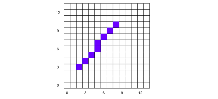
Suppose we have two points P1 = (2, 3) and P2 = (10, 8). We want to draw a straight line between these two points using the DDA algorithm.
Let's understand its step-by-step process.
Calculate the slope mmm
$$\mathrm{m = \frac{y_2 - y_1}{x_2 - x_1} = \frac{8 - 3}{10 - 2} = \frac{5}{8} = 0.625}$$
Since the slope m ≤ 1, we increment the x-coordinate by 1 unit at each step. Now follow the following table for a detailed steps −
Find the increments
- We set Δx = 1 because we are incrementing the x-coordinate by 1.
- The corresponding increment in y is given by: Δy = m × Δx = 625 × 1 = 0.625
Starting Point
The starting point is (x1, y1) = (2, 3). Begin plotting the line from this point.
Next Point
Increment the x-coordinate by 1 and add Δy to the current y-value. Keep track of both values.
- New x: x1 + 1 = 2 + 1 = 3
- New y: y1 + Δy = 3 + 0.625 = 3.625 round to 4
Thus the points are forming −
| Step | x | y | Pixel |
|---|---|---|---|
| 0 | 2.000 | 3.000 | (2, 3) |
| 1 | 2.857 | 4.000 | (3, 4) |
| 2 | 3.714 | 5.000 | (4, 5) |
| 3 | 4.571 | 6.000 | (5, 6) |
| 4 | 5.429 | 7.000 | (5, 7) |
| 5 | 6.286 | 8.000 | (6, 8) |
| 6 | 7.143 | 9.000 | (7, 9) |
| 7 | 8.000 | 10.000 | (8, 10) |
Advantages of the DDA Algorithm
The DDA algorithm is simple and easy to implement. It works efficiently for lines with a gentle slope (less than or equal to 1). Since it uses floating-point arithmetic, it produces smooth lines, but we need to round them off for pixels. It is an incremental algorithm, which means the calculations are done step by step.
Disadvantages of the DDA Algorithm
The main disadvantage of the DDA algorithm is its reliance on floating-point arithmetic, which can be slower on some systems. Floating-point operations tend to be more computationally expensive than integer operations. Additionally, rounding operations can introduce small errors in the plotted line, which may lead to inaccuracies over long distances.
Conclusion
In this chapter, we have seen the idea of DDA algorithm in detail to draw straight lines between two points. We started by understanding the basic concept of the algorithm, followed by a detailed explanation of how it works. We also walked through a step-by-step example of plotting a line between two points.
The DDA algorithm is efficient for simple line drawing tasks and is easy to implement. However, it may not be the best choice for all situations due to its use of floating-point arithmetic.