Scan Line Algorithm for Polygon Filling in Computer Graphics

---

---

The scanline algorithm is an efficient method for filling polygons with color. This algorithm works by dividing the polygon into horizontal lines, called scanlines. Filling the pixels between pairs of intersections.

Read this chapter to learn how the Scanline Polygon Filling Algorithm works. We will also see its components, and walk through an example to understand the process for a better understanding.

Basics of Scanline Polygon Filling

Scanline filling is the process of coloring the interior pixels of a polygon by using horizontal lines, known as scanlines. The algorithm operates by moving from the bottom of the polygon to the top, line by line.

At each scanline, it checks for intersections with the polygon's edges. When a scanline intersects with a polygon edge, the algorithm determines the region between pairs of intersections and fills it with color.

How Does Scanline Work?

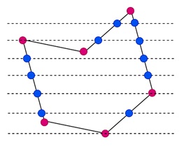
To visualize the Scanline Algorithm, imagine that we are drawing a line on paper using a single pen. We begin at the left border of the shape to the right and if there are intersection in between, do not draw the line at the point. The algorithm is working in the similar way. In the following figure, the same is being reflected. Red dots are polygon points and blue dots are intersection points on the polygon.

Special Cases of Polygon Vertices

There are special cases to consider when the scanline intersects the vertices of a polygon −

• Same-Side Intersections − If both lines that meet at the vertex are on the same side of the scanline, the vertex is treated as two points.
• Opposite-Side Intersections − If the lines intersecting at the vertex are on opposite sides of the scanline, the vertex is considered as only one point.

These rules ensure that the polygon is filled correctly without any gaps or overlapping regions.

Data-structure of Scanline Polygon Filling Algorithm

The Scanline Algorithm consists of several data structures that work together to fill the polygon. These components are −

• Edge Buckets − Edge buckets hold data about each polygon edge. They contain important details like the maximum y-coordinate (yMax), the x-coordinate of the lowest point (xOfYmin), and the inverse slope of the edge (slopeInverse).
• Edge Table (ET) − The edge table holds all the edges of the polygon in lists. Each list corresponds to a specific scanline, and the edges in the list are ordered based on the yMin values of the edges. The edge table helps in organizing the edges so they can be processed efficiently, scanline by scanline.
• Active List (AL) − The active list is responsible for keeping track of the current edges that are being used to fill the polygon. Edges are added to the active list from the edge table when their yMin value matches the current scanline. The active list is updated and re-sorted after each scanline is processed.

Example

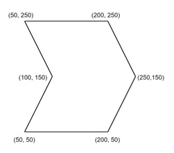
Consider the polygon with points (50, 50), (200, 50), (250, 150), (200, 250), (50, 250), (100, 150). The polygon is looking like −

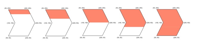
The polygon filling is looking like −

Scanline Filling Algorithm: Step by Step

Let us see how scanline polygon filling algorithm in detail −

Store Polygon Edges

First, we process each polygon edge and store its information in the edge table. The information stored includes the yMax, xOfYmin, and slopeInverse of each edge.

Order and Sort Edges

The edges are ordered based on their yMin values, meaning the edges are sorted according to the y-coordinate of their lowest point. Within each scanline, the edges are sorted by their xOfYmin values using insertion sort. This ensures that the edges are processed from left to right.

Start Filling

Once the edge table is fully populated, the filling process begins from the bottom scanline (the scanline with the smallest y-coordinate). The process continues scanline by scanline until the top of the polygon is reached.

Active List Management

At each scanline, the active edge list (AL) is updated. The edges whose yMin matches the current scanline are added to the active list. After updating, the active list is sorted by the xOfYmin values.

Remove Completed Edges

If an edge’s yMax value is equal to or less than the current scanline, that edge is removed from the active list. This is because the edge is no longer relevant for further scanlines.

Filling between Pairs of Edges

Once the active list is sorted, the algorithm pairs up the edges and fills the pixels between them.

If a vertex is encountered, the following rules are applied:

• If both intersecting lines at the vertex are on the same side of the scanline, the vertex is treated as two points.
• If the intersecting lines are on opposite sides of the scanline, the vertex is treated as one point.

Update xOfYmin

After each scanline is processed, the xOfYmin values of the edges in the active list are updated by adding the slopeInverse of the edge. This ensures that the edges move correctly to the next scanline.

Repeat Until Complete

The process is repeated for every scanline, and the polygon is filled completely once all the edges are removed from the edge table.

Conclusion

The scanline polygon filling algorithm is an efficient method for filling polygons. In this chapter, we explained its basic concepts, how the algorithm works, and how the special cases of polygon vertices are handled. There are several data-structures to design this algorithm.