Computer Graphics Surfaces

---

---

Polygon Surfaces

Objects are represented as a collection of surfaces. 3D object representation is divided into two categories.

• Boundary Representations (B-reps) − It describes a 3D object as a set of surfaces that separates the object interior from the environment.

• Spacepartitioning representations − It is used to describe interior properties, by partitioning the spatial region containing an object into a set of small, non-overlapping, contiguous solids (usually cubes).

The most commonly used boundary representation for a 3D graphics object is a set of surface polygons that enclose the object interior. Many graphics system use this method. Set of polygons are stored for object description. This simplifies and speeds up the surface rendering and display of object since all surfaces can be described with linear equations.

The polygon surfaces are common in design and solid-modeling applications, since their wireframe display can be done quickly to give general indication of surface structure. Then realistic scenes are produced by interpolating shading patterns across polygon surface to illuminate.

Polygon Tables

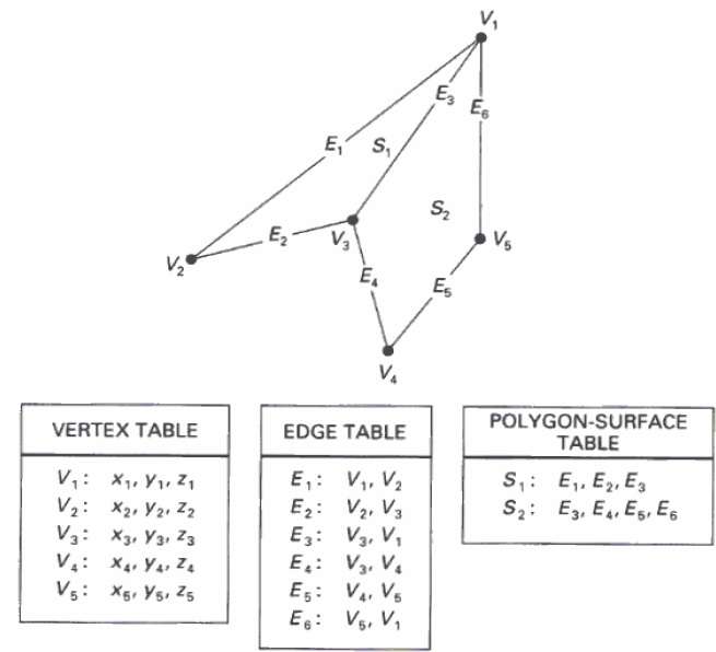
In this method, the surface is specified by the set of vertex coordinates and associated attributes. As shown in the following figure, there are five vertices, from v₁ to v₅.

• Each vertex stores x, y, and z coordinate information which is represented in the table as v₁: x₁, y₁, z₁.

• The Edge table is used to store the edge information of polygon. In the following figure, edge E₁ lies between vertex v₁ and v₂ which is represented in the table as E₁: v₁, v₂.

• Polygon surface table stores the number of surfaces present in the polygon. From the following figure, surface S₁ is covered by edges E₁, E₂ and E₃ which can be represented in the polygon surface table as S₁: E₁, E₂, and E₃.

Plane Equations

The equation for plane surface can be expressed as −

Ax + By + Cz + D = 0

Where (x, y, z) is any point on the plane, and the coefficients A, B, C, and D are constants describing the spatial properties of the plane. We can obtain the values of A, B, C, and D by solving a set of three plane equations using the coordinate values for three non collinear points in the plane. Let us assume that three vertices of the plane are (x₁, y₁, z₁), (x₂, y₂, z₂) and (x₃, y₃, z₃).

Let us solve the following simultaneous equations for ratios A/D, B/D, and C/D. You get the values of A, B, C, and D.

(A/D) x₁ + (B/D) y₁ + (C/D) z₁ = -1

(A/D) x₂ + (B/D) y₂ + (C/D) z₂ = -1

(A/D) x₃ + (B/D) y₃ + (C/D) z₃ = -1

To obtain the above equations in determinant form, apply Cramers rule to the above equations.

$A = \begin{bmatrix} 1& y_{1}& z_{1}\\ 1& y_{2}& z_{2}\\ 1& y_{3}& z_{3} \end{bmatrix} B = \begin{bmatrix} x_{1}& 1& z_{1}\\ x_{2}& 1& z_{2}\\ x_{3}& 1& z_{3} \end{bmatrix} C = \begin{bmatrix} x_{1}& y_{1}& 1\\ x_{2}& y_{2}& 1\\ x_{3}& y_{3}& 1 \end{bmatrix} D = - \begin{bmatrix} x_{1}& y_{1}& z_{1}\\ x_{2}& y_{2}& z_{2}\\ x_{3}& y_{3}& z_{3} \end{bmatrix}$

For any point (x, y, z) with parameters A, B, C, and D, we can say that −

• Ax + By + Cz + D ≠ 0 means the point is not on the plane.

• Ax &plus; By &plus; Cz &plus; D < 0 means the point is inside the surface.

• Ax &plus; By &plus; Cz &plus; D > 0 means the point is outside the surface.

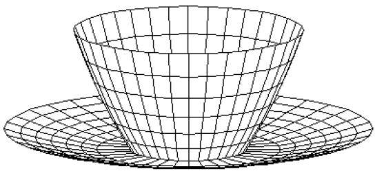
Polygon Meshes

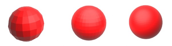
3D surfaces and solids can be approximated by a set of polygonal and line elements. Such surfaces are called polygonal meshes. In polygon mesh, each edge is shared by at most two polygons. The set of polygons or faces, together form the skin of the object.

This method can be used to represent a broad class of solids/surfaces in graphics. A polygonal mesh can be rendered using hidden surface removal algorithms. The polygon mesh can be represented by three ways −

• Explicit representation
• Pointers to a vertex list
• Pointers to an edge list

Advantages

• It can be used to model almost any object.
• They are easy to represent as a collection of vertices.
• They are easy to transform.
• They are easy to draw on computer screen.

Disadvantages

• Curved surfaces can only be approximately described.
• It is difficult to simulate some type of objects like hair or liquid.