Specular Reflection Models in Computer Graphics

---

---

Different models help achieve realistic visual effects by approximating the behavior of light in various conditions. Specular reflection simulates how light reflects off surfaces.

In this chapter, we will discuss the basics of specular reflection models, along with detailed examples to understand their application. We will also focus on the mathematical formulations for a better understanding.

What is Specular Reflection?

Specular reflection deals with light reflecting off a surface in a single direction, much like a mirror. The appearance and intensity of these reflections depend on several factors. These are the properties of the material, the angle of incidence, and the surface smoothness.

Specular reflection models are often represented using the Bidirectional Reflectance Distribution Function (BRDF). This defines how light is reflected at different angles.

In computer graphics, these models simulate materials such as metals, plastics, and glass. Each type of material has unique properties that affect the way it interacts with light. understanding.

Specular Reflection Models

There are several models used for simulating specular reflection. This section we will see some of the basic models and their applications.

Lambertian Model

The Lambertian model is one of the simplest models for light reflection. It assumes that light is scattered equally in all directions. In terms of the BRDF, a Lambertian surface has a constant reflectance value. It does not change with viewing angle.

This model is often used to simulate diffuse surfaces like chalk or matte paper. For example, if the BRDF is Lambertian, then the ideal Probability Density Function (pdf) is proportional to cos(θ). This leads to the equation as follows −

$$\mathrm{p(k) \:=\: \frac{1}{\pi} \cos \theta}$$

This model is not suitable for surfaces that exhibit glossy or mirror-like reflections.

Schlicks Approximation

The Schlick's approximation is a method used to simulate the Fresnel effect. Here it describes how the reflectance changes with the angle of incidence. For a metal, the reflectance at normal incidence, denoted as R0 it is typically used.

The formula for reflectance based on Schlicks approximation is −

$$\mathrm{R(\theta,\: \lambda) \:=\: R_0(\lambda) \:+\: (1 \:+\: R_0(\lambda)) (1 \:-\: \cos \theta)^5}$$

This approximation helps artists and programmers to set the normal reflectance of the material from data or by visual approximation.

There are materials like dielectrics (glass, water), on which this can be applied. The formula can be adjusted using the refractive index n −

$$\mathrm{R_0(\lambda) \:=\: \left( \frac{n(\lambda) \:-\: 1}{n(\lambda) \:+\: 1} \right)^2}$$

This helps to simulate materials like water with n = 1.33 or glass with n = 1.4 to n = 1.7.

Smooth-Layered Model

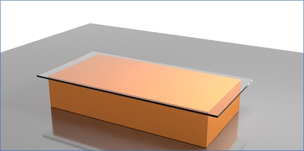
The smooth-layered model is used for materials like polished woods or plastics, where reflection occurs at the surface and scattering within the subsurface. The smooth surface reflects light according to the Fresnel equations. The subsurface scattering affects the light that is transmitted through the surface.

The reflectance changes with viewing angle due to these interactions. For example, when simulating polished tiles, a Monte Carlo path tracer can be used to generate images.

The reflectance of the smooth surface can be calculated as −

$$\mathrm{\rho(\theta,\: \phi,\: \theta',\: \phi',\: \lambda) \:=\: R_f(\theta)\: \rho_s(\theta,\: \phi,\: \theta',\: \phi') \:+\: \frac{R_d(\lambda)}{\pi}}$$

Here, R_f(θ) is the Fresnel reflectance and ρ_s is the normalized specular BRDF.

Coupled Model for Matte and Specular Tradeoff

Multiple materials may be coupled with. The coupled model may addresses the matte and specular tradeoff by combining the behavior of matte and specular reflection. It maintains energy conservation and reciprocity. This means that the amount of energy reflected is equal to the amount of energy absorbed. This model is useful for surfaces with both matte and glossy characteristics.

For example, in the coupled model, the BRDF is defined as −

$$\mathrm{\rho(\theta,\: \phi,\: \theta',\: \phi',\: \lambda) \:=\: R_f(\theta)\: \rho_s(\theta,\: \phi,\: \theta',\: \phi') \:+\: k R_m(\lambda) \left[ 1 \:-\: R_f(\theta) \right]\: \left[ 1 \:-\: R_f(\theta') \right]}$$

This formula is used to compute the tradeoff between the matte and specular reflections. The key parameter R_f(θ) is derived from the Fresnel equations.

Rough-Layered Model

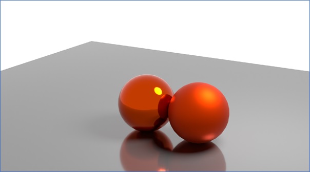
Another type of material is the rough-layered model. It is an extension of the coupled model for surfaces that are not perfectly smooth. It introduces a spread in the specular component to account for surface roughness.

This model is particularly useful for simulating metals, plastics, and other common materials. For example, the rough-layered model uses an anisotropic specular BRDF, where the reflectance varies based on the surface orientation.

The BRDF is expressed as −

$$\mathrm{\rho(k_1,\: k_2) \:=\: \frac{(n_u \:+\: 1)(n_v \:+\: 1)}{8\pi} \frac{(n \:\cdot\: h)^{n_u} \cos^2 \phi \:+\: n_v \sin^2 \phi}{(h \:\cdot\: k_i) \max(\cos \theta_i,\: \cos \theta_o)} F(k_i,\: h)}$$

This equation is used for modeling metallic surfaces with varying degrees of roughness.

Practical Applications of Specular Reflection Models

Specular reflection models have practical applications in rendering realistic scenes in computer graphics. They are widely used in game development, movies, and simulation software to achieve realistic materials and lighting. Artists and engineers can adjust the parameters like the refractive index and reflectance to achieve the desired visual effects.

In a gaming environment, a rough-layered model can be used to simulate surfaces like brushed metals or rough plastics. For smooth surfaces like glass, the smooth-layered model is more appropriate.

Conclusion

In this chapter, we explained the various specular reflection models used in computer graphics. These include the Lambertian model, Schlick’s approximation, smooth-layered model, coupled model, and rough-layered model.

These models are used to simulate the complex behavior of light on different materials. They help rendered scenes look more realistic.