Computer Graphics - Line Generation Algorithm

---

---

A line connects two points. It is a basic element in graphics. To draw a line, you need two points between which you can draw a line. In the following three algorithms, we refer the one point of line as $X_{0}, Y_{0}$ and the second point of line as $X_{1}, Y_{1}$.

DDA Algorithm

Digital Differential Analyzer (DDA) algorithm is the simple line generation algorithm which is explained step by step here.

Step 1 − Get the input of two end points $(X_{0}, Y_{0})$ and $(X_{1}, Y_{1})$.

Step 2 − Calculate the difference between two end points.

dx = X1 - X0
dy = Y1 - Y0

Step 3 − Based on the calculated difference in step-2, you need to identify the number of steps to put pixel. If dx > dy, then you need more steps in x coordinate; otherwise in y coordinate.

if (absolute(dx) > absolute(dy))
   Steps = absolute(dx);
else
   Steps = absolute(dy);

Step 4 − Calculate the increment in x coordinate and y coordinate.

Xincrement = dx / (float) steps;
Yincrement = dy / (float) steps;

Step 5 − Put the pixel by successfully incrementing x and y coordinates accordingly and complete the drawing of the line.

for(int v=0; v < Steps; v++)
{
   x = x + Xincrement;
   y = y + Yincrement;
   putpixel(Round(x), Round(y));
}

Bresenham's Line Generation

The Bresenham algorithm is another incremental scan conversion algorithm. The big advantage of this algorithm is that, it uses only integer calculations. Moving across the x axis in unit intervals and at each step choose between two different y coordinates.

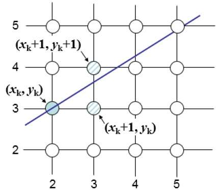
For example, as shown in the following illustration, from position (2, 3) you need to choose between (3, 3) and (3, 4). You would like the point that is closer to the original line.

At sample position $X_{k}+1,$ the vertical separations from the mathematical line are labelled as $d_{upper}$ and $d_{lower}$.

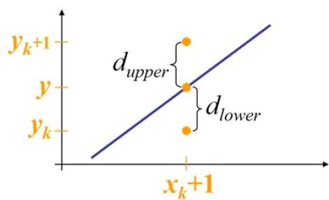
From the above illustration, the y coordinate on the mathematical line at $x_{k}+1$ is −

Y = m($X_{k}$+1) + b

So, $d_{upper}$ and $d_{lower}$ are given as follows −

$$d_{lower} = y-y_{k}$$

$$= m(X_{k} + 1) + b - Y_{k}$$

and

$$d_{upper} = (y_{k} + 1) - y$$

$= Y_{k} + 1 - m (X_{k} + 1) - b$

You can use these to make a simple decision about which pixel is closer to the mathematical line. This simple decision is based on the difference between the two pixel positions.

$$d_{lower} - d_{upper} = 2m(x_{k} + 1) - 2y_{k} + 2b - 1$$

Let us substitute m with dy/dx where dx and dy are the differences between the end-points.

$$dx (d_{lower} - d_{upper}) =dx(2\frac{\mathrm{d} y}{\mathrm{d} x}(x_{k} + 1) - 2y_{k} + 2b - 1)$$

$$ = 2dy.x_{k} - 2dx.y_{k} + 2dy + 2dx(2b-1)$$

$$ = 2dy.x_{k} - 2dx.y_{k} + C$$

So, a decision parameter $P_{k}$ for the kth step along a line is given by −

$$p_{k} = dx(d_{lower} - d_{upper})$$

$$ = 2dy.x_{k} - 2dx.y_{k} + C$$

The sign of the decision parameter $P_{k}$ is the same as that of $d_{lower} - d_{upper}$.

If $p_{k}$ is negative, then choose the lower pixel, otherwise choose the upper pixel.

Remember, the coordinate changes occur along the x axis in unit steps, so you can do everything with integer calculations. At step k+1, the decision parameter is given as −

$$p_{k +1} = 2dy.x_{k + 1} - 2dx.y_{k + 1} + C$$

Subtracting $p_{k}$ from this we get −

$$p_{k + 1} - p_{k} = 2dy(x_{k + 1} - x_{k}) - 2dx(y_{k + 1} - y_{k})$$

But, $x_{k+1}$ is the same as $(xk)+1$. So −

$$p_{k+1} = p_{k} + 2dy - 2dx(y_{k+1} - y_{k})$$

Where, $Y_{k+1} Y_{k}$ is either 0 or 1 depending on the sign of $P_{k}$.

The first decision parameter $p_{0}$ is evaluated at $(x_{0}, y_{0})$ is given as −

$$p_{0} = 2dy - dx$$

Now, keeping in mind all the above points and calculations, here is the Bresenham algorithm for slope m < 1 −

Step 1 − Input the two end-points of line, storing the left end-point in $(x_{0}, y_{0})$.

Step 2 − Plot the point $(x_{0}, y_{0})$.

Step 3 − Calculate the constants dx, dy, 2dy, and (2dy 2dx) and get the first value for the decision parameter as −

$$p_{0} = 2dy - dx$$

Step 4 − At each $X_{k}$ along the line, starting at k = 0, perform the following test −

If $p_{k}$ < 0, the next point to plot is $(x_{k}+1, y_{k})$ and

$$p_{k+1} = p_{k} + 2dy$$ Otherwise,

$$(x_{k}, y_{k}+1)$$

$$p_{k+1} = p_{k} + 2dy - 2dx$$

Step 5 − Repeat step 4 (dx 1) times.

For m > 1, find out whether you need to increment x while incrementing y each time.

After solving, the equation for decision parameter $P_{k}$ will be very similar, just the x and y in the equation gets interchanged.

Mid-Point Algorithm

Mid-point algorithm is due to Bresenham which was modified by Pitteway and Van Aken. Assume that you have already put the point P at (x, y) coordinate and the slope of the line is 0 ≤ k ≤ 1 as shown in the following illustration.

Now you need to decide whether to put the next point at E or N. This can be chosen by identifying the intersection point Q closest to the point N or E. If the intersection point Q is closest to the point N then N is considered as the next point; otherwise E.

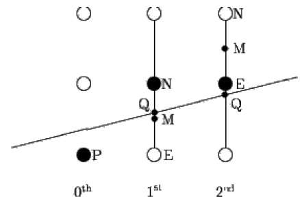
To determine that, first calculate the mid-point M(x+1, y + ½). If the intersection point Q of the line with the vertical line connecting E and N is below M, then take E as the next point; otherwise take N as the next point.

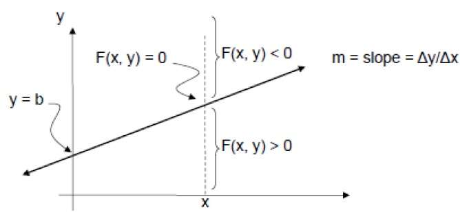
In order to check this, we need to consider the implicit equation −

F(x,y) = mx + b - y

For positive m at any given X,

• If y is on the line, then F(x, y) = 0
• If y is above the line, then F(x, y) < 0
• If y is below the line, then F(x, y) > 0