Transformation Between Coordinate System in Computer Graphics

---

---

When we apply the rotation matrix, it rotates on the origin itself. When working with 3D models or 2D shapes, it's important to understand how these objects can be moved, rotated, and resized. To change their transformation with some other pivot points, we can change the coordinate points itself. These operations are typically done by transforming their coordinates from one system to another.

In this chapter, we will explain the basics of coordinate system transformations with the help of a set of examples for a better understanding.

Basics of Coordinate Systems

A coordinate system is a reference framework that defines the position of points in space. In 2D graphics, this framework usually consists of two perpendicular axes: x (horizontal) and y (vertical). In 3D graphics, an additional z-axis is added to represent depth.

Suppose we have a previous coordinate system like −

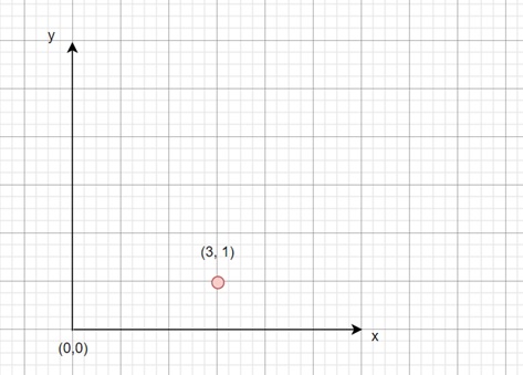
When we work with objects in computer graphics, they are usually defined in their own local coordinate system. However, to display these objects on a screen, we need to transform their coordinates into a global coordinate system or world coordinate system. This transformation allows us to position, rotate, or scale objects relative to the global scene.

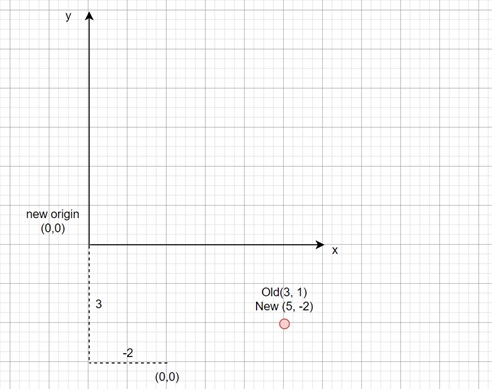
Let us understand the effect of coordinate transformation in true sense. Consider the above point. Initially the coordinate system is at origin (0, 0) and the point is at (3, 1). Now if we shift the coordinate system origin to (-2, 3), then the new coordinate for the point will be (5, -2). So, the new center (h, k) is (-2, 3) as per the old coordinate systems. But considering this as the new origin, it is at (0, 0) and the given point is at −

$$\mathrm{\left( 3 \:-\: (-2),\: 1 \:-\: 3 \right) \:=\: \left( 5,\: -2 \right)}$$

Coordinate Transformation Matrices

To transform coordinates between different systems, we use transformation matrices. These matrices help us change the position, scale, or orientation of an object. In 2D, we use a 3x3 matrix, while in 3D, we use a 4x4 matrix.

For example, a 2D transformation matrix looks like this −

$$\mathrm{\left[ \begin{array}{ccc} a_{11} & a_{12} & t_x \\ a_{21} & a_{22} & t_y \\ 0 & 0 & 1 \end{array} \right]}$$

Here, the elements a₁₁ , a₁₂, a₂₁ and a₂₂ represent scaling and rotation, while t_x and t_y represent the translation along the x and y axes. The third row ensures the transformation works properly with homogeneous coordinates.

Local vs Global Coordinate Systems

In graphics applications, it is common to manage objects in local or object coordinate systems. These systems describe an object's geometry relative to its own origin. For example, when modelling a car, the local coordinate system would be centered around the car itself. The car's parts would be positioned relative to this local origin.

However, to render the car in a scene, we must place it in the global coordinate system, which represents the overall scene or world. In this system, other objects like trees, roads, or trees also exist.

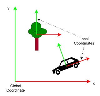
Here, we have the global position for the tree and the car, but based on their local system they have separate coordinates. The car is tilted, but according to its local system it is not tilted. In other words the base of the car is always parallel to the local x axis.

Example of Transforming a Point

Let us go through an example to make the concept clearer. Consider a point (2, 1) in a 2D local coordinate system. We want to apply a transformation that translates the point by (1, 0), moving it one unit to the left. This transformation is represented by the following matrix −

$$\mathrm{\left[ \begin{array}{ccc} 1 & 0 & -1 \\ 0 & 1 & 0 \\ 0 & 0 & 1 \end{array} \right]}$$

When this matrix is multiplied by the point [2, 1, 1]^T, it produces the new coordinates (1, 1). This means the point has been moved left by one unit.

But, this transformation can be interpreted in two ways −

• Moving the point − We think of this transformation as physically moving the point itself from (2, 1) to (1, 1)
• Changing the coordinate system − Instead of moving the point, we could think of the transformation as shifting the entire coordinate system. In this case, the point remains in the same location relative to its system, but the system itself moves.

Both interpretations lead to the same result mathematically, but thinking in terms of coordinate system changes can often make transformations easier to understand, especially when managing complex scenes with multiple objects.

Transformation of Multiple Objects

Let us consider a more complex scenario where multiple objects need to be transformed. If you think the above example with a tree and a car, extend this to a driving game, where the player controls a car. The car is moving through a way, and we need to transform the trees and streets to reflect the car's movement.

In this case, we apply transformations to each trees and street object. We can think of this as either moving the objects relative to the car or moving the coordinate system attached to the car itself. Each object, like a tree or a street, is transformed in a way that makes it appear to move backward as the car moves forward.

If the player switches to an overhead view to see the car's position in the city, the transformation works in the opposite way. Now, the car is moved relative to the city, and the trees and streets remain fixed in their positions. The same transformation matrix is applied, but the way we interpret the movement depends on whether the objects are in the car's local coordinate system or the city's global coordinate system.

Conclusion

In this chapter, we explained basics of coordinate systems and how the local and global systems work. We covered how transformation matrices are used to move, scale, and rotate objects within these systems. We then went through examples like translating a point, moving multiple objects in a game, and we explained how to manage multiple objects movement effectively.