B-Spline Curves and Surfaces in Computer Graphics

---

---

B-Spline curves are widely used in creating smooth and flexible shapes. B-Spline curves offer two key advantages over Bzier curves. First, the degree of the B-Spline polynomial can be set independently of the number of control points. Second, B-Splines allow local control, meaning we can modify part of the curve without affecting the rest.

Read this chapter to understand B-Spline curves and surfaces, their properties, and how they differ from other types of curves.

What is B-Spline Curve?

A B-Spline curve, short for Basis Spline, is a smooth curve defined by a set of control points. The curve does not necessarily pass through these control points but is influenced by their positions. This allows for more control and flexibility when designing curves in computer graphics.

Advantages of B-Spline Curves

Following are the advantages of using B-Spline Curves −

• Degree Independence − Unlike Bezier curves, the degree of a B-Spline curve can be set independently of the number of control points. This provides more freedom in designing curves.
• Local Control − One of the key advantages of B-Spline curves is their ability to offer local control. This means that modifying one part of the curve does not affect the other parts. We can change a control point and only influence the curve's nearby section without altering the entire curve.

General Expression for B-Spline Curves

Let us see the equation for a B-Spline curve −

$$\mathrm{p(k) = \sum_{k=0}^{n} p_k B_{k,d}(u), \quad u_{\text{min}} \leq u \leq u_{\text{max}}, \quad 2 \leq d \leq n+1}$$

Where,

• p_k represents the control points.
• B_(k,d)(u) is the B-Spline blending function.
• u is a parameter that ranges between minimum and maximum values depending on the chosen B-Spline parameters.

The blending function, B_(k,d) (u), is a polynomial of degree d-1. The degree d can be set to any value between 2 and n + 1, where n is the number of control points. If d is set to 1, the curve becomes a simple point set."

Local Control in B-Spline Curves

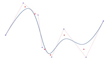
One of the most powerful features of B-Spline curves is their local control. Adjusting a local control point, we can change part of the curve without affecting the rest. For example, if we modify one control point in a curve with several control points, only the part of the curve near that control point changes, while the rest of the curve remains the same.

Properties of B-Spline Curves

B-Spline curves have several important properties −

Degree of the Curve

The degree of a B-Spline curve is d-1, where d is the degree of the polynomial used in the blending function.

Control Point Influence

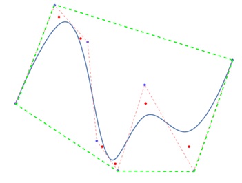
A B-Spline curve lies within the convex hull of its control points. This means the curve will follow the general path outlined by the control points but will remain inside the convex polygon formed by them. In the following figure, green dashed lines are forming convex hull.

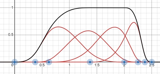
Blending Function and Local Control

The blending function in a B-Spline curve is defined recursively using the Cox-Deboor recursion formula. The blending function helps in defining how much influence each control point has on the curve.

The formula is as follows −

$$\mathrm{B_{k,1}(u) \:=\: \begin{cases} 1, & \text{if } u_k \leq u \leq u_{k+1} \\ 0, & \text{otherwise} \end{cases}}$$

$$\mathrm{B_{k,1}(u)\: =\: \frac{u \:-\: u_k}{u_{k\:+\:d\:-\:1} \:-\: u_k} B_{k,\:d\:-\:1}(u)\: +\: \frac{u_{k\:+\:d} \:-\: u}{u_{k\:+\:d} \:-\: u_{k+1}} B_{k+1,\:d-1}(u)}$$

Where,

• u_krepresents the knot values in the knot vector.
• d is the degree of the curve.

Convex Hull Property

The curve is tightly bounded by the control points and stays within the convex hull formed by the control points. This is similar to Bezier curve. We have seen in the above figure.

Adding or Removing Control Points

A B-Spline curve allows us to add or remove control points without changing the degree of the curve. This feature makes B-Splines very flexible in design.

Tight Fit to Control Points

The B-Spline curve follows the control points closely, but it is influenced by the control points within a certain range, allowing for smooth transitions.

Knot Vector

The values that define the intervals of influence for the blending functions are called knot vectors. The knot values in the knot vector must follow the rule −

$$\mathrm{u_j\: \leq\: u_{j+1}}$$

This ensures that the curve progresses smoothly through the control points without any sudden jumps.

Uniform, Open Uniform, and Non-Uniform B-Splines

B-Splines can be classified into three categories based on the arrangement of the knot vectors −

• Uniform B-Spline
• Open Uniform B-Spline
• Non-Uniform B-Spline

Uniform B-Spline

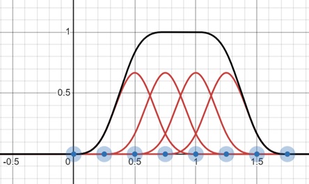
In a uniform B-Spline, the spacing between the knot values is constant. This creates a periodic blending function. All blending functions have the same shape and are simply shifted versions of each other.

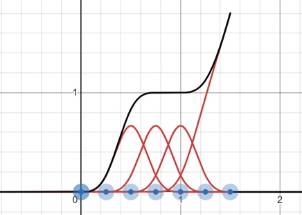
Open Uniform B-Spline

In an open uniform B-Spline, the first and last knot values are repeated. This ensures that the curve passes through the first and last control points.

Non-Uniform B-Spline

In non-uniform B-Splines, the spacing between the knot values is not constant. This allows for more flexibility in controlling the shape of the curve but requires more computation.

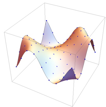
B-Spline Surfaces

B-Spline surfaces are an extension of B-Spline curves into three dimensions. A B-Spline surface is defined by a grid of control points, and the surface is influenced by these points.

Like B-Spline curves, B-Spline surfaces offer local control and flexibility in design. They are widely used in 3D modeling applications, especially for creating smooth and complex surfaces such as car bodies, furniture, and other objects that require precise control.

The equation for B-Spline surface is similar to the curve.

$$\mathrm{P(u,v) \:=\: \sum_{i=0}^{n} \sum_{j=0}^{m} p_{i,j} B_{i,p}(u) B_{j,q}(v)}$$

Here B_i,p(u) and B_j,q(v) are B-spline basis functions of degree p and q, respectively.

Properties of B-Spline Surfaces

Local Control − Similar to the curve, B-Spline surfaces offer local control. You can modify part of the surface without affecting the entire shape.

• Tight Fit to Control Points − The surface lies within the convex hull of the control points, following their general shape.
• Flexible Design − B-Spline surfaces can be created with any number of control points and offer more flexibility than other surface representation methods.

Conclusion

In this chapter, we covered the B-Spline curves and surfaces, highlighting their properties, advantages, and how they are used in computer graphics.

We started by explaining what B-Spline curves are and how they offer degree independence and local control. We then understood important properties such as convex hull, blending functions, and the knot vector.

We also discussed the different types of B-Splines, including uniform, open uniform, and non-uniform B-Splines. Finally, we understood B-Spline surfaces, which extend B-Splines into three dimensions for modelling complex shapes.