- Computer Graphics - Home
- Computer Graphics Basics
- Computer Graphics Applications
- Graphics APIs and Pipelines
- Computer Graphics Maths
- Sets and Mapping
- Solving Quadratic Equations
- Computer Graphics Trigonometry
- Computer Graphics Vectors
- Linear Interpolation
- Computer Graphics Devices
- Cathode Ray Tube
- Raster Scan Display
- Random Scan Device
- Phosphorescence Color CRT
- Flat Panel Displays
- 3D Viewing Devices
- Images Pixels and Geometry
- Color Models
- Line Generation
- Line Generation Algorithm
- DDA Algorithm
- Bresenham's Line Generation Algorithm
- Mid-point Line Generation Algorithm
- Circle Generation
- Circle Generation Algorithm
- Bresenham's Circle Generation Algorithm
- Mid-point Circle Generation Algorithm
- Ellipse Generation Algorithm
- Polygon Filling
- Polygon Filling Algorithm
- Scan Line Algorithm
- Flood Filling Algorithm
- Boundary Fill Algorithm
- 4 and 8 Connected Polygon
- Inside Outside Test
- 2D Transformation
- 2D Transformation
- Transformation Between Coordinate System
- Affine Transformation
- Raster Methods Transformation
- 2D Viewing
- Viewing Pipeline and Reference Frame
- Window Viewport Coordinate Transformation
- Viewing & Clipping
- Point Clipping Algorithm
- Cohen-Sutherland Line Clipping
- Cyrus-Beck Line Clipping Algorithm
- Polygon Clipping Sutherland–Hodgman Algorithm
- Text Clipping
- Clipping Techniques
- Bitmap Graphics
- 3D Viewing Transformation
- 3D Computer Graphics
- Parallel Projection
- Orthographic Projection
- Oblique Projection
- Perspective Projection
- 3D Transformation
- Rotation with Quaternions
- Modelling and Coordinate Systems
- Back-face Culling
- Lighting in 3D Graphics
- Shadowing in 3D Graphics
- 3D Object Representation
- Represnting Polygons
- Computer Graphics Surfaces
- Visible Surface Detection
- 3D Objects Representation
- Computer Graphics Curves
- Computer Graphics Curves
- Types of Curves
- Bezier Curves and Surfaces
- B-Spline Curves and Surfaces
- Data Structures For Graphics
- Triangle Meshes
- Scene Graphs
- Spatial Data Structure
- Binary Space Partitioning
- Tiling Multidimensional Arrays
- Color Theory
- Colorimetry
- Chromatic Adaptation
- Color Appearance
- Antialiasing
- Ray Tracing
- Ray Tracing Algorithm
- Perspective Ray Tracing
- Computing Viewing Rays
- Ray-Object Intersection
- Shading in Ray Tracing
- Transparency and Refraction
- Constructive Solid Geometry
- Texture Mapping
- Texture Values
- Texture Coordinate Function
- Antialiasing Texture Lookups
- Procedural 3D Textures
- Reflection Models
- Real-World Materials
- Implementing Reflection Models
- Specular Reflection Models
- Smooth-Layered Model
- Rough-Layered Model
- Surface Shading
- Diffuse Shading
- Phong Shading
- Artistic Shading
- Computer Animation
- Computer Animation
- Keyframe Animation
- Morphing Animation
- Motion Path Animation
- Deformation Animation
- Character Animation
- Physics-Based Animation
- Procedural Animation Techniques
- Computer Graphics Fractals
Mid-point Line Generation Algorithm
The Mid-Point Line Drawing Algorithm is used to draw straight lines between two points on a pixel grid using mid-point finding approach. It is popular because it is both efficient and simple. In this chapter, we will explain the internal details of this algorithm with examples for a better understanding.
Mid-point Line Generation Algorithm
The main idea of the Mid-Point Line Drawing Algorithm is to find the best pixels to make a straight line. It does this by choosing the next pixel closest to the ideal line at each step. This method keeps the line looking accurate. The algorithm uses integer math. This makes it work well, even on systems that are not very powerful.
We must follow a set of concepts to understand this algorithm well. These are listed below
- Pixel Selection − The algorithm looks at the mid-point between two possible pixel positions. It then uses a decision variable to pick the pixel that is closest to the actual line.
- Decision Variable − This variable helps decide which pixel is closer to the line. It is updated with each step to show how much error has built up. This guides the choice of the next pixel.
- Incremental Error Calculation − Instead of calculating the line equation over and over, the algorithm updates the error bit by bit. This makes the algorithm work faster.
Algorithm Steps
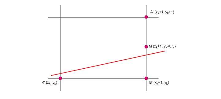
- Initialization − First, we find the differences Δx and Δy between the start point (x0, y0) and the end point (x1, y1). Then we set the initial decision variable d based on the midpoint rule.
-
Iterative Drawing − For each pixel from start to end:
- Plot the pixel at (x, y)
- Update the decision variable d
- Choose the next pixel based on d −
- If d is less than 0, move right
- If not, move diagonally up and right
- Updating the Decision Variable: Update the decision variable d based on how the error changes when we move to the next pixel.
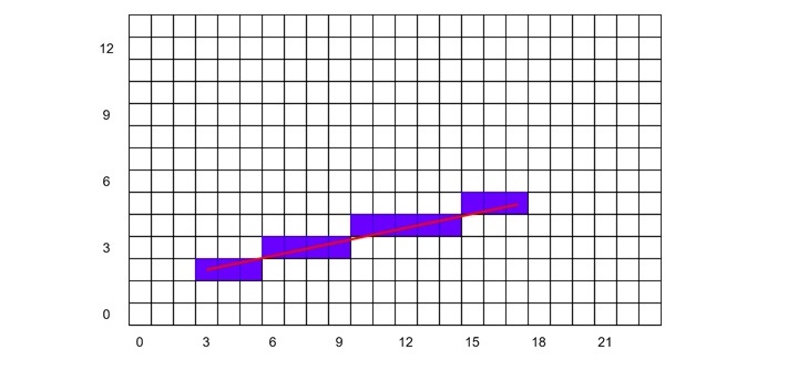
Example 1
Let us take an example to demonstrate how this algorithm works.
Consider the input points (3, 2) and (17, 5).
| Step | x | y | D | Action | Plot Point |
|---|---|---|---|---|---|
| Init | 3 | 2 | dy - (dx / 2) = 3 - (14 / 2) = -4 | Initialize values | (3, 2) |
| 1 | 4 | 2 | d + dy = -4 + 3 = -1 | Increment x | (4, 2) |
| 2 | 5 | 2 | d + dy = -1 + 3 = 2 | Increment x | (5, 2) |
| 3 | 6 | 3 | d + (dy - dx) = 2 + (3 - 14) = -9 | Increment x, y | (6, 3) |
| 4 | 7 | 3 | d + dy = -9 + 3 = -6 | Increment x | (7, 3) |
| 5 | 8 | 3 | d + dy = -6 + 3 = -3 | Increment x | (8, 3) |
| 6 | 9 | 3 | d + dy = -3 + 3 = 0 | Increment x | (9, 3) |
| 7 | 10 | 4 | d + (dy - dx) = 0 + (3 - 14 ) = -11 | Increment x, y | (10, 4) |
| 8 | 11 | 4 | d + dy = -11 + 3 = -8 | Increment x | (11, 4) |
| 9 | 12 | 4 | d + dy = -8 + 3 = -5 | Increment x | (12, 4) |
| 10 | 13 | 4 | d + dy = -5 + 3 = -2 | Increment x | (13, 4) |
| 11 | 14 | 4 | d + dy = -2 + 3 = 1 | Increment x | (14, 4) |
| 12 | 15 | 5 | d + (dy - dx) = 1 + (3 - 14) = -10 | Increment x, y | (15, 5) |
| 13 | 16 | 5 | d + dy = -10 + 3 = -7 | Increment x | (16, 5) |
| 14 | 17 | 5 | d + dy = -7 + 3 = -4 | Increment x | (17, 5) |
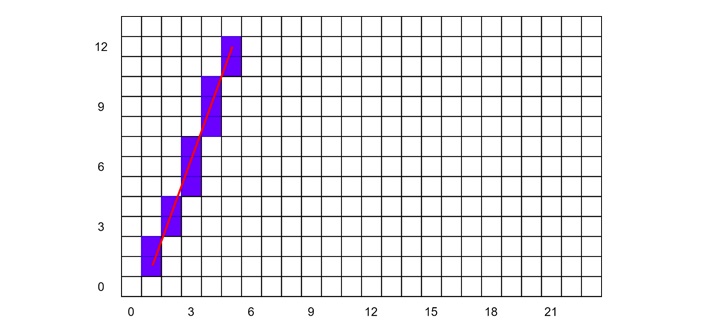
Example 2
Let us see another example. Consider the input points (1, 1) and (5, 12).
| Step | x | y | d | Action | Plot Point |
|---|---|---|---|---|---|
| Init | 1 | 1 | d = dy - (dx / 2) = 11 - (4 / 2) = 9 | Initialize values | (1, 1) |
| 1 | 1 | 2 | d + (dy - dx) = 9 + (11 - 4) = 16 | Increment y | (1, 2) |
| 2 | 2 | 3 | d - dx = 16 - 4 = 12 | Increment x, y | (2, 3) |
| 3 | 2 | 4 | d - dx = 12 - 4 = 8 | Increment y | (2, 4) |
| 4 | 3 | 5 | d - dx = 8 - 4 = 4 | Increment x, y | (3, 5) |
| 5 | 3 | 6 | d - dx = 4 - 4 = 0 | Increment y | (3, 6) |
| 6 | 3 | 7 | d - dx = 0 - 4 = -4 | Increment y | (3, 7) |
| 7 | 4 | 8 | d + (dy - dx) = -4 + (11 - 4) = 3 | Increment x, y | (4, 8) |
| 8 | 4 | 9 | d - dx = 3 - 4 = -1 | Increment y | (4, 9) |
| 9 | 4 | 10 | d - dx = -1 - 4 = -5 | Increment y | (4, 10) |
| 10 | 5 | 11 | d + (dy - dx) = -5 + (11 - 4) = 2 | Increment x, y | (5, 11) |
| 11 | 5 | 12 | d - dx = 2 - 4 = -2 | Increment y | (5, 12) |
Advantages of the Mid-Point Algorithm
Like Bresenham's algorithm this is also efficient since it uses only integer math. This makes it fast. It produces lines that look smooth and accurate. And the algorithm is easy to understand and implement.
Conclusion
In this chapter, we explained the Mid-Point Line Drawing Algorithm in detail. We covered how it works to draw straight lines on pixel grids. We highlighted the key concepts like pixel selection and the decision variable.
We also presented two detailed examples, showing how to draw a line. We explained in detail how the algorithm makes decisions at each step to choose the best pixels.