Shading in Ray Tracing

---

---

Shading helps us simulate how light interacts with surfaces to create realistic images. Without shading effect, 3D objects look dull. With ray tracing, we can calculate the lighting of each pixel based on the intersection of rays and objects.

In this chapter, we will discuss different shading models, how they work, and their impact in creating realistic images. We will cover the basics of shading, along with specific examples like Lambertian, Blinn-Phong, and ambient shading.

Basics of Shading in Ray Tracing

Shading in ray tracing can be done once we know which surface a ray intersects. The pixel value is then computed by evaluating a shading model. The shading model can range from simple heuristics to complex numerical computations.

Most shading models are designed to capture the process of light reflection. This is when surfaces are illuminated by light sources and reflect part of the light to the camera.

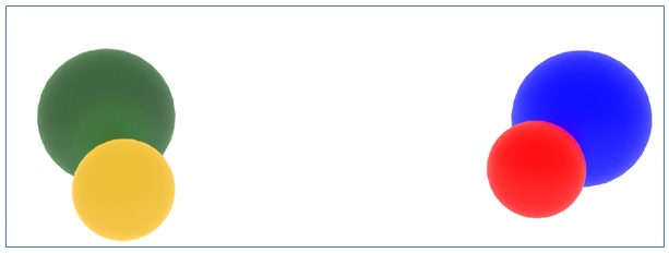
Take a look at the following image; here we haven't applied any shading.

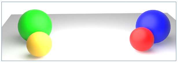
Now see the following image where shading is applied.

There are three main elements in shading −

• Light direction
• View direction
• Surface normal

Each of these is represented by a unit vector. The light direction points towards the light source, the view direction points towards the camera, and the surface normal is perpendicular to the surface at the point where reflection happens. These vectors, along with the surface properties like color and shininess, determine how a surface appears when illuminated. Let us see some shading types.

Lambertian Shading

The simplest shading model is the Lambertian shading model. It is named after Johann Heinrich Lambert, who observed that the energy from a light source falling on a surface depends on the angle between the light and the surface.

A surface facing directly towards the light gets maximum illumination. If the surface is tangent to the light or faces away from it, it receives no illumination. The illumination is proportional to the cosine of the angle between the surface normal and the light direction.

The Lambertian shading model can be expressed as −

$$\mathrm{L \:=\: k_d \:\cdot\: I \:\cdot\: \max(0,\: n\: \cdot\: l)}$$

Where,

• L is the pixel color.
• k_d is the diffuse coefficient or surface color.
• I is the intensity of the light source.
• n is the surface normal vector.
• l is the light direction vector.

The dot product n⋅ l represents the cosine of the angle between the surface normal and the light. This model is often used to create a matte or chalky appearance on surfaces, as it does not produce highlights or shininess.

Blinn-Phong Shading

Next shading technique is Blinn-Phong Shading. Lambertian shading is useful for matte surfaces, but many real-world surfaces are shiny. Shiny surfaces produce highlights, which can be simulated with the Blinn-Phong shading model. This model adds a specular component to the Lambertian shading. It was developed by Jim Blinn as an update to the Phong shading model.

The Blinn-Phong shading model determines how bright the reflection will be when the view direction and light direction are symmetric around the surface normal. It uses a half-vector h, which is the bisector of the angle between the view and light directions. The reflection is brightest when h and n (the surface normal) are aligned. The brightness decreases as h moves away from n.

The Blinn-Phong shading model is given as −

$$\mathrm{L \:=\: k_d \:\cdot\: I \:\cdot\: \max(0,\: n \:\cdot\: l) \:+\: k_s \:\cdot\: l \:\cdot\: \max(0,\: n \:\cdot\: h)^p}$$

Where,

• k_s is the specular coefficient or surface shininess.
• h is the half-vector, calculated as $\mathrm{h = \frac{v + l}{|v + l|}}$.
• p is the Phong exponent, which controls how shiny the surface appears.

The power p controls the appearance of the highlight. Small values of p create wide, soft highlights, while large values create tight, bright highlights. The Blinn-Phong shading model is suitable for surfaces like metal or polished materials.

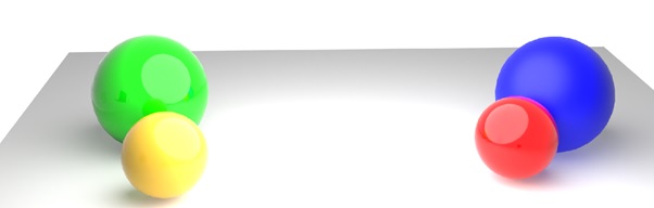
See the spheres except the blue one with gloss effect.

Ambient Shading

Another shading type for the real-world objects are rarely illuminated by direct light alone. They also receive light reflected from other surfaces. In ray tracing, we simulate this with ambient shading. Ambient shading adds a constant amount of light to all surfaces, regardless of their position or orientation. This prevents surfaces that are not directly lit from appearing completely black.

The ambient shading model can be written as −

$$\mathrm{L \:=\: k_a \:\cdot\: I_a}$$

Where,

• L is the pixel color.
• k_a is the ambient coefficient, representing how much ambient light the surface reflects.
• I_a is the intensity of the ambient light.

Ambient shading is often combined with other models like Lambertian and Blinn-Phong. Together, these models form a complete shading equation −

$$\mathrm{L \:=\: k_a \:\cdot\: I_a \:+\: k_d \:\cdot\: I \:\cdot\: \max(0,\: n \:\cdot\: l) \:+\: k_s \:\cdot\: I \:\cdot\: \max(0,\: n \:\cdot\: h)^p}$$

This equation takes into account ambient light, diffuse reflection, and specular reflection, making it a simple yet effective model for many shading scenarios.

Multiple Point Lights

In realistic scenes, there are usually multiple light sources. The effects of multiple lights can be computed using the property of superposition. This means the total illumination is the sum of the illumination caused by each light source individually.

The shading equation for N light sources becomes −

$$\mathrm{L \:=\: k_a \:\cdot\: I_a \:+\: \sum_{i=1}^{N} \left[ k_d \:\cdot\: I_i \:\cdot\: \max(0, \:n \:\cdot\: l_i)\: +\: k_s \:\cdot\: I_i \:\cdot\: \left( \max(0,\: n \:\cdot\: h_i) \right)^p \right]}$$

Where,

• I_i is the intensity of the i-th light source.
• l_i is the light direction for the i-th light source.
• h_i is the half-vector for the i-th light source.

Using multiple light sources allows for more complex and realistic lighting effects in ray tracing.

Implementing Shading in Ray Tracing

To implement shading in ray tracing, we first generate a viewing ray for each pixel. Then, we find the intersection of the ray with the nearest object. Once we have the intersection point and the surface normal, we evaluate the shading model to determine the pixel color.

for each pixel do
   compute viewing ray
   if (ray hits an object):
      compute surface normal
      evaluate shading model
      set pixel color to the computed color
   else:
      set pixel color to background color

This process shows that each pixel is colored based on the lighting and material properties of the surfaces it intersects. It also handles shadows and occlusions to make the image more realistic.

Conclusion

In this chapter, we explained the shading techniques in ray tracing. We covered the basics of shading and explored the different models like Lambertian, Blinn-Phong, and ambient shading. In addition, we explained how to handle multiple light sources and how to implement these models in a ray-tracing program.