Bezier Curves and Surfaces in Computer Graphics

---

---

It was Pierre Bezier, a French engineer, who popularized Bezier Curves for designing automobile bodies at Renault. Bezier curves are widely used in various CAD (Computer-Aided Design) and graphics software due to their flexibility and ease of implementation.

Read this chapter to learn what Bezier curves are, their properties, and how they are used in design. We will also discuss Bezier surfaces for a better understanding.

What are Bezier Curves?

Bezier curves are parametric curves that can be fitted to any number of control points. These control points are used to shape the curve and determine its degree. The degree of a Bezier curve is always one less than the number of control points.

For example, if there are three control points, the Bezier curve will be of degree two; if there are four control points, the curve will be of degree three, and so on.

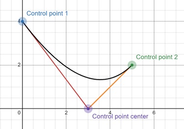
The quadratic (degree 2) Bezier curve is like with three control points −

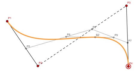
The cubic Bezier curve is like −

Example

The Bezier curve equation is defined using a blending function. This blending function helps combine the control points to form the curve. A Bezier curve can be represented as −

$$\mathrm{P(u) \:=\: \sum_{k=0}^{n} p_k \: \text{BEZ}_{k,n}(u), \quad 0 \:\leq \:u\: \leq\: 1}$$

Where,

• p_k represents the control points.
• BEZ_k,n) (u) is the blending function.
• u is a parameter that varies between 0 and 1, controlling the position along the curve.

Bezier Blending Function

The Bezier blending function is crucial for creating the curve. It is calculated using the binomial coefficient, also known as C(n, k), which you may remember from high school math. The blending function is defined as:

$$\mathrm{\text{BEZ}_{k,n}(u) \:=\: C(n,k) u^k (1\:-\:u)^{n-k}}$$

Where C(n, k) is the binomial coefficient, calculated as −

$$\mathrm{C(n,k) \:=\: \frac{n!}{k! \, (n \:-\: k)!}}$$

This blending function ensures that the curve smoothly follows the control points.

Properties of Bezier Curves

Bezier curves have several important properties that make them useful in computer graphics:

Start and End Points

A Bezier curve always passes through its first and last control points. For example, if the first control point is P0 and the last control point is Pn, the curve starts at P0 and ends at Pn.

First-Order Derivative

The parametric first-order derivative of a Bezier curve at the start and end points can be calculated using the control points. At the starting point, the derivative is −

$$\mathrm{p'(0) \:=\: -n\: \cdot\: p_0 \:+\: n\: \cdot\: p_1}$$

At the end point, the derivative is −

$$\mathrm{p'(1) \:=\: -n \:\cdot\: p_{n-1} \:+\: n\: \cdot\: p_n}$$

Second-Order Derivative

The second-order derivative of a Bezier curve can also be calculated. At the starting point, the second-order derivative is −

$$\mathrm{p''(0) \:=\: n\: \cdot\: (n \:-\: 1)\: \cdot\: \left[ (p_2 \:-\: p_1) \:-\: (p_1 \:-\: p_0) \right]}$$

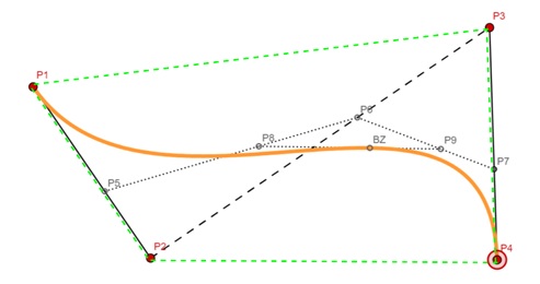
Convex Hull Property

A Bezier curve always lies within the convex hull of its control points. This means the curve will not stray outside the polygon formed by the control points. In the following figure, green dashed lines are convex hull.

Blending Function Positivity

The Bezier blending function is always positive, meaning the weights applied to the control points will always be positive. This ensures a smooth curve.

Sum of Blending Functions

The sum of all Bezier blending functions for a curve always equals 1. This property states that the curve is correctly defined by the control points:

$$\mathrm{\sum_{k=0}^{n} \text{BEZ}_{k,n}(u) \:=\: 1}$$

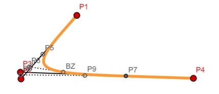
Weighted Control Points

Any point on the Bezier curve is a weighted sum of the control points. If two control points are placed at the same position, the curve will be pulled more strongly toward that position due to the increased weight.

In the figure, two points P2 and P3 are very close (not at the same position due to picture clarity) the curve is much more bended at that part.

Smoothness of Bezier Curves

A Bezier curve smoothly follows the control points without erratic oscillations. This makes it designing smooth shapes.

High-Degree Bezier Curves

While Bezier curves can be fitted to any number of control points, increasing the number of control points also increases the polynomial degree of the curve. Higher-degree curves require more computational power because they involve more complex calculations.

To solve this problem, complicated Bezier curves can be divided into smaller sections of lower-order Bezier curves. Each section can be designed separately, giving better control over the shape of the curve and reducing computational complexity.

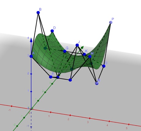
Bezier Surfaces

Just as Bezier curves are used to create smooth lines, Bezier surfaces are used to create smooth surfaces in 3D graphics. A Bezier surface is defined by a grid of control points, and the surface is shaped according to these points. Bezier surfaces are widely used in 3D modelling and CAD software to create smooth, organic shapes.

Equation for the Bezier surface is quite similar to the curve −

$$\mathrm{P(u,v) \:=\: \sum_{i=0}^{n} \sum_{j=0}^{m} p_{i,j} \: \text{BEZ}_{i,n}(u) \: \text{BEZ}_{j,m}(v), \quad 0\: \leq\: u,\:v\: \leq\: 1}$$

Where,

• $\mathrm{p_{i,j}}$ represents the control points.
• $\mathrm{BEZ_{i,n} (u)}$ and $\mathrm{BEZ_{j,m} (v)}$ are the blending function.
• u,v are parameters that varies between 0 and 1, controlling the position along the curve.
• $\mathrm{BEZ_{i,n} (u) \:=\: C(n,i) u^i (1\:-\:u)^{n-i}}$
• $\mathrm{BEZ_{j,m} (v) \:=\: C(m,j) v^j (1\:-\:v)^{m-j}}$

Properties of Bezier Surfaces

Bezier surfaces share many of the same properties as Bezier curves, including −

• They pass through the first and last control points.
• The surface lies within the convex hull of the control points.
• The blending functions used to define the surface are positive.

Bezier surfaces are especially useful for designing complex shapes like car bodies, furniture, and other objects that require smooth, flowing surfaces.

Conclusion

In this chapter, we explained in detail the Bezier curves and surfaces, their properties, equations, and their applications in computer graphics.

We started by discussing how Bezier curves work, including how they are defined by control points and blending functions. We also looked at the important properties of Bezier curves, such as their smoothness, ability to pass through control points, and how they can be shaped by adjusting control points.

Finally, we understood Bezier surfaces, which extend Bezier curves into 3D space. This allows designers to create smooth, complex surfaces.