Computer Graphics - Circle Generation Algorithm

---

---

Drawing a circle on the screen is a little complex than drawing a line. There are two popular algorithms for generating a circle − Bresenhams Algorithm and Midpoint Circle Algorithm. These algorithms are based on the idea of determining the subsequent points required to draw the circle. Let us discuss the algorithms in detail −

The equation of circle is $X^{2} + Y^{2} = r^{2},$ where r is radius.

Bresenham's Algorithm

We cannot display a continuous arc on the raster display. Instead, we have to choose the nearest pixel position to complete the arc.

From the following illustration, you can see that we have put the pixel at (X, Y) location and now need to decide where to put the next pixel − at N (X+1, Y) or at S (X+1, Y-1).

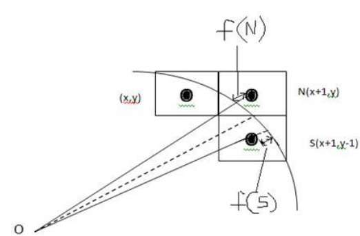
This can be decided by the decision parameter d.

• If d <= 0, then N(X+1, Y) is to be chosen as next pixel.
• If d > 0, then S(X+1, Y-1) is to be chosen as the next pixel.

Algorithm

Step 1 − Get the coordinates of the center of the circle and radius, and store them in x, y, and R respectively. Set P=0 and Q=R.

Step 2 − Set decision parameter D = 3 2R.

Step 3 − Repeat through step-8 while P ≤ Q.

Step 4 − Call Draw Circle (X, Y, P, Q).

Step 5 − Increment the value of P.

Step 6 − If D < 0 then D = D + 4P + 6.

Step 7 − Else Set R = R - 1, D = D + 4(P-Q) + 10.

Step 8 − Call Draw Circle (X, Y, P, Q).

Draw Circle Method(X, Y, P, Q).

Call Putpixel (X + P, Y + Q).
Call Putpixel (X - P, Y + Q).
Call Putpixel (X + P, Y - Q).
Call Putpixel (X - P, Y - Q).
Call Putpixel (X + Q, Y + P).
Call Putpixel (X - Q, Y + P).
Call Putpixel (X + Q, Y - P).
Call Putpixel (X - Q, Y - P).

Mid Point Algorithm

Step 1 − Input radius r and circle center $(x_{c,} y_{c})$ and obtain the first point on the circumference of the circle centered on the origin as

(x0, y0) = (0, r)

Step 2 − Calculate the initial value of decision parameter as

$P_{0}$ = 5/4 r (See the following description for simplification of this equation.)

f(x, y) = x2 + y2 - r2 = 0

f(xi - 1/2 + e, yi + 1)
        = (xi - 1/2 + e)2 + (yi + 1)2 - r2 
        = (xi- 1/2)2 + (yi + 1)2 - r2 + 2(xi - 1/2)e + e2
        = f(xi - 1/2, yi + 1) + 2(xi - 1/2)e + e2 = 0

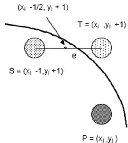
Let di = f(xi - 1/2, yi + 1) = -2(xi - 1/2)e - e2
Thus,

If e < 0 then di > 0 so choose point S = (xi - 1, yi + 1).
di+1    = f(xi - 1 - 1/2, yi + 1 + 1) = ((xi - 1/2) - 1)2 + ((yi + 1) + 1)2 - r2
        = di - 2(xi - 1) + 2(yi + 1) + 1
        = di + 2(yi + 1 - xi + 1) + 1
		  
If e >= 0 then di <= 0 so choose point T = (xi, yi + 1)
   di+1 = f(xi - 1/2, yi + 1 + 1)
       = di + 2yi+1 + 1
		  
The initial value of di is
   d0 = f(r - 1/2, 0 + 1) = (r - 1/2)2 + 12 - r2
      = 5/4 - r {1-r can be used if r is an integer}
		
When point S = (xi - 1, yi + 1) is chosen then
   di+1 = di + -2xi+1 + 2yi+1 + 1
	
When point T = (xi, yi + 1) is chosen then
   di+1 = di + 2yi+1 + 1

Step 3 − At each $X_{K}$ position starting at K=0, perform the following test −

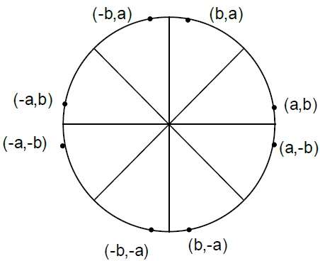
If PK < 0 then next point on circle (0,0) is (XK+1,YK) and
   PK+1 = PK + 2XK+1 + 1
Else
   PK+1 = PK + 2XK+1 + 1  2YK+1
	
Where, 2XK+1 = 2XK+2 and 2YK+1 = 2YK-2.

Step 4 − Determine the symmetry points in other seven octants.

Step 5 − Move each calculate pixel position (X, Y) onto the circular path centered on $(X_{C,} Y_{C})$ and plot the coordinate values.

X = X + XC,   Y = Y + YC

Step 6 − Repeat step-3 through 5 until X >= Y.