Ray-Object Intersection in Ray Tracing

---

---

An important aspect of Ray Tracing is determining where the rays intersect with the objects in the scene. In this chapter, we will explain the process of ray-object intersection in ray tracing. We will focus on the interaction between rays and spheres, triangles, and polygons. We will see the mathematical formulations and examples for a better understanding.

Basics of Ray-Object Intersection

The primary task in ray tracing is to find the intersection of a ray with an object. Suppose we have a ray of the form.

$$\mathrm{p(t) \:=\: e \:+\: t\: \cdot \:d}$$

where e is the ray's origin and d is its direction, the goal is to find points where the ray intersects the surfaces of objects in the scene. This is solving an equation for t, where t > 0.

In ray-object intersection, we sometimes use more general technique to solve. Find intersections within a specific interval [t0, t1]. The simplest case is when t0 = 0 and t1 = +∞. This interval can be adjusted depending on the application and specific intersection requirements.

Ray-Sphere Intersection

Let us start intersection from spheres. To find where a ray intersects with a sphere, we begin with the ray equation −

$$\mathrm{p(t) \:=\: e \:+\: t \:\cdot\: d}$$

A sphere can be represented by the implicit equation −

$$\mathrm{(x \:-\: xc)^2 \:+\: (y \:-\: yc)^2 \:+\: (z \:-\: zc)^2 \:-\: R^2 \:=\: 0}$$

where (xc, yc, zc) is the center of the sphere and R is its radius. This equation can also be written in vector form as:

$$\mathrm{(p \:-\: c) \:\cdot\: (p \:-\: c) \:-\: R^2 \:=\: 0}$$

Next, substitute the ray equation into the sphere equation to get an equation in terms of t −

$$\mathrm{(e \:+\: t d \:-\: c) \:\cdot\: (e \:+\: t d \:-\: c) \:-\: R^2 \:=\: 0}$$

Simplifying further, we get a quadratic equation −

$$\mathrm{(d \:\cdot\: d) t^2 \:+\: 2d \:\cdot\: (e \:-\: c) t \:+\: (e \:-\: c)^2 \:-\: R^2 \:=\: 0}$$

where,

A = d · d

B = 2d · (e - c)

C = (e - c) · (e - c) - R².

$$\mathrm{}$$

Solving for t, we use the quadratic formula −

$$\mathrm{t \:=\: \frac{-B \:\pm \sqrt{B^2 \:-\: 4AC}}{2A}}$$

The discriminant B² − 4AC determines the number of intersections. If the discriminant is negative, the ray does not intersect the sphere. If it is positive, there are two solutions: one where the ray enters the sphere and one where it exits. If the discriminant is zero, the ray just grazes the sphere at one point.

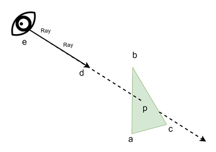
Ray-Triangle Intersection

Ray-triangle intersections are calculated using a system of linear equations. Given the vertices of a triangle a, b, and c, we set up the intersection equation −

$$\mathrm{e \:+\: t d \:=\: a \:+\: \beta (b \:-\: a) \:+ \:\gamma (c \:-\: a)}$$

where t, β, and γ are unknowns.

The ray hits the triangle if β > 0, γ > 0, and β + γ < 1.

We can expand this equation into three separate equations for the x, y, and z-coordinates:

$$\mathrm{x_e \:+\: t x_d \:=\: x_a \:+\: \beta (x_b \:-\: x_a) \:+\: \gamma (x_c \:-\: x_a)}$$

$$\mathrm{y_e \:+\: t y_d \:=\: y_a \:+\: \beta (y_b \:-\: y_a) \:+\: \gamma (y_c \:-\: y_a)}$$

$$\mathrm{z_e \:+\: t z_d \:=\: z_a \:+\: \beta (z_b \:-\: z_a) \:+\: \gamma (z_c \:-\: z_a)}$$

These three equations can be solved as a linear system using Cramers rule. The linear system can be represented as a matrix equation −

$$\mathrm{A \:\begin{bmatrix} \beta \\ \gamma \\ t \end{bmatrix} \:=\: \begin{bmatrix} x_a \:-\: x_e \\ y_a \:-\: y_e \\ z_a \:-\: z_e \end{bmatrix}}$$

where matrix A contains the coefficients of β, γ, and t. Solving this system will return values of β, γ, and t.

Ray-Polygon Intersection

Next, another type is for a polygon with m vertices, ray-polygon intersection is computed by first finding the intersection of the ray with the plane containing the polygon. This is done using the equation of a plane −

$$\mathrm{(p \:-\: p_1) \:\cdot\: n \:=\: 0}$$

where p1 is any vertex of the polygon and n is the surface normal.

Solving for t, we get −

$$\mathrm{t \:=\: \frac{(p_1 \:-\: e) \:\cdot\: n}{d \:\cdot\: n}}$$

If t is positive, we compute the point p where the ray intersects the plane. Then, we check if p is inside the polygon. This can be done by projecting p and the polygon vertices onto the xyplane and counting the intersections between a ray from p and the polygon edges.

Intersecting a Group of Objects

In real-world scenes, multiple objects exist. Finding the intersection of a ray with a group of objects involves checking each object individually and keeping track of the closest intersection point.

For a group of objects, a simple approach is to iterate over each object and find the intersection with the smallest t-value. This ensures that the ray hits the nearest object.

for each object in the group:
    if (object is hit at ray parameter t and t ∈ [t0, t1]):
        keep track of the smallest t value
return the closest intersection

This method is efficient determination of ray intersections in complex scenes with multiple objects.

Conclusion

In this chapter, we covered the concept of ray-object intersections in ray tracing. We understood ray intersection on sphere, triangle, and polygon in detail. Each type of intersection was explained with equations and conditions necessary to find solutions. Additionally, we understood how to handle multiple objects in a scene which is necessary for real-world scenario.