Affine Transformation in Computer Graphics

---

---

There are different types of transformations that we can apply on points; affine transformation is one of them. It is widely used to manipulate objects within a 2D or 3D space. These transformations help to perform essential transformations like rotating, scaling, and translating objects.

In this chapter, we will cover the basics of affine transformation, explain how they work, and go through a detailed example for a better understanding.

Basics of Affine Transformation

An affine transformation is a transformation that preserves points, straight lines, and planes. When applying affine transformations, parallel lines remain parallel, but angles between lines or the lengths of the lines may not be preserved.

Affine transformations can be described using matrices, which allows for easy computation and combination of multiple transformations. Some of these transformations are −

• Translation − Moving an object from one position to another without rotating or scaling it.
• Rotation − Rotating an object around a point.
• Scaling − Increasing or decreasing the size of an object.
• Shearing − Slanting the shape of an object.

We can apply affine transformations using matrix multiplications. And this makes it possible to apply efficiently in any points or polygons.

Matrix Representation of Affine Transformation

To perform affine transformations, we typically use a matrix. For 2D transformations, the matrix is a 33 matrix. The general form of a 2D affine transformation matrix is −

$$\mathrm{\left[ \begin{array}{ccc} m_{11} & m_{12} & t_x \\ m_{21} & m_{22} & t_y \\ 0 & 0 & 1 \end{array} \right]}$$

Here, the elements m₁₁, m₁₂, m₂₁ and m₂₂ represent scaling and rotation, while t_x and t_y represent translation along the X and Y axes. The last row ensures that we are working with homogeneous coordinates, which we will explain further.

In a traditional 2D transformation, we use a 2×2 matrix. However, this matrix cannot handle translations with multiplication. That’s why we extend the transformation to a 3×3 matrix and represent points in 2D space as a 3D vector by adding a third coordinate.

For example, a point (x, y) becomes [x, y, 1]^T. The transformation matrix can then be applied to this vector, and the resulting vector will include the transformed X and Y coordinates along with a 1.

Homogeneous Coordinates

Here is an interesting concept called the homogeneous coordinates. To make translation possible using matrix multiplication, we introduce homogeneous coordinates. Homogeneous coordinates add an extra dimension to points, allowing translation to be treated like scaling and rotation.

Consider a point (x, y) in 2D space. In homogeneous coordinates, we represent this point as [x, y, 1]^T. A 3×3 matrix that performs a translation can now move the point in space without needing to handle the translation separately. This method combines translation, scaling, and rotation into a single matrix operation.

For example, the matrix for translation by (t_x, t_y) looks like this −

$$\mathrm{\left[ \begin{array}{ccc} 1 & 0 & t_x \\ 0 & 1 & t_y \\ 0 & 0 & 1 \end{array} \right]}$$

When we multiply this matrix by the point [x, y, 1]^T, the result is [x + t_x, y + t_y, 1]^T, which translates the point.

Example of Affine Transformation

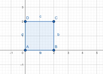
Let us see the affine transformations in action. Suppose we have a square (polygon) with its endpoints at A = (0, 0), B = (2, 0), C = (2, 2), D = (0, 2). We will apply the transformations one by one to get the final figures.

Now let us apply translation, where we use (t_x, t_y) as translation parameters. With (t_x, t_y) = (5, 3) the final shape will be −

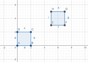
Here, ABCD is the previous polygon and EFGH is the polygon after translation.

$$\mathrm{\text{Translation Matrix} = \left[ \begin{array}{ccc} 1 & 0 & 5 \\ 0 & 1 & 3 \\ 0 & 0 & 1 \end{array} \right]}$$

The next affine transformation is rotation. Here, we are applying rotation of 135 degrees on ABCD, and resultant polygon is ABCD. The rotation is happening on pivot at (0, 0) coordinate.

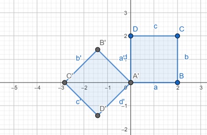
$$\mathrm{\text{Rotation Matrix} = \left[ \begin{array}{ccc} \cos(\theta) & -\sin(\theta) & 0 \\ \sin(\theta) & \cos(\theta) & 0 \\ 0 & 0 & 1 \end{array} \right] = \left[ \begin{array}{ccc} \cos(135^\circ) & -\sin(135^\circ) & 0 \\ \sin(135^\circ) & \cos(135^\circ) & 0 \\ 0 & 0 & 1 \end{array} \right]}$$

Next is scaling. For this we need scaling factors. For two axes the scaling factors are s_x and s_y. The s_x is scaling factor for X-axis and s_y for Y-axis. Let us see the matrix and corresponding action.

$$\mathrm{\text{Scaling Matrix} = \left[ \begin{array}{ccc} s_x & 0 & 0 \\ 0 & s_y & 0 \\ 0 & 0 & 1 \end{array} \right]}$$

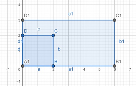
Here, we are considering s_x = 3 and s_y = 1.5.

$$\mathrm{\left[ \begin{array}{ccc} s_x & 0 & 0 \\ 0 & s_y & 0 \\ 0 & 0 & 1 \end{array} \right] = \left[ \begin{array}{ccc} 3 & 0 & 0 \\ 0 & 1.5 & 0 \\ 0 & 0 & 1 \end{array} \right]}$$

Here A1, B1, C1 and D1 is forming the scaled polygon.

Let us now see the other transformation called shearing. Here too, we need two parameters: sh_x and sh_y. sh_x is shearing parameter along the X-axis and sh_y is shearing parameter along the Y-axis. Let us see the matrix and their effect.

$$\mathrm{\text{Shearing Matrix} = \left[ \begin{array}{ccc} 1 & sh_x & 0 \\ sh_y & 1 & 0 \\ 0 & 0 & 1 \end{array} \right]}$$

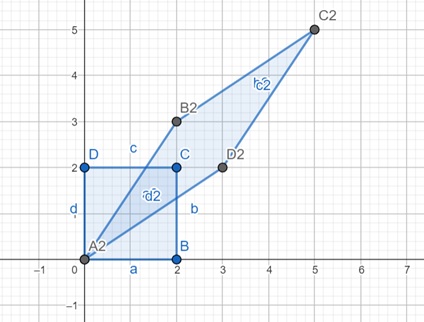
We are taking sh_x = 1.5 and sh_y = 1.5. The final shape is looking like the above figure and the points are A2, B2, C2 and D2.

$$\mathrm{\left[ \begin{array}{ccc} 1 & sh_x & 0 \\ sh_y & 1 & 0 \\ 0 & 0 & 1 \end{array} \right] = \left[ \begin{array}{ccc} 1 & 1.5 & 0 \\ 1.5 & 1 & 0 \\ 0 & 0 & 1 \end{array} \right]}$$

Affine Transformation in 3D

Affine transformations also extend naturally to three dimensions (3D). In 3D, we use a 4x4 matrix instead of a 3x3 matrix. The basic operations (translation, rotation, scaling, shearing) still apply, but now we must account for the z-dimension as well.

For example, the matrix for translating a point (x, y, z) by (t_x, t_y, t_z) is:

$$\mathrm{\left[ \begin{array}{cccc} 1 & 0 & 0 & t_x \\ 0 & 1 & 0 & t_y \\ 0 & 0 & 1 & t_z \\ 0 & 0 & 0 & 1 \end{array} \right]}$$

In this matrix, the extra row and column handle the z-dimension, and points in 3D space are represented as [x, y, z, 1]^T.

Conclusion

In this chapter, we explained the basics of affine transformation in computer graphics. We discussed what affine transformations are and how they are represented using matrices. We also explained homogeneous coordinates and how they enable translation in the matrix framework. We then looked at an example of affine transformations including translation, rotation, scaling and shearing.