Antialiasing Texture Lookups for Texture Mapping

---

---

In texturing, we sometimes need antialiasing techniques to make the graphics visually correct. Aliasing is a significant problem of textures. Aliasing occurs when high-frequency details in the texture cause unwanted artifacts like jagged edges or shimmering. To prevent these issues, we use antialiasing. Antialiasing effects make the texture look smooth and visually appealing, even at different distances or angles.

In this chapter, we will see how antialiasing is applied to texture lookups. We will explore the key concepts like pixel footprints and discuss techniques like mipmapping, etc.

Antialiasing in Texture Mapping

Antialiasing is used in rendering a texture-mapped image is a sampling process. When a texture is mapped onto a 3D surface, it creates a 2D function across the image plane. This is sampled at pixels.

Using simple point samples to render this 2D function can create aliasing artifacts, especially when the image has sharp edges or fine details. Since the primary purpose of textures is to introduce these details, textures can easily become a source of aliasing problems.

To solve this issue, we need to compute each pixels value as an area average, rather than as a point sample. It means the pixel color should be based on an average of the texture colors over an area that corresponds to the pixel size.

Pixel Footprint in Texture Mapping

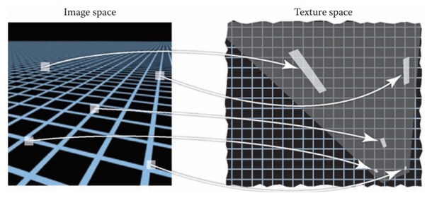
The relationship between the image and the texture is constantly changing during rendering. Every pixel value should be an average color over the area that the pixel covers on the surface. When the surface color comes from a texture. This is nothing but averaging over a corresponding area in the texture. This area is known as the texture space footprint of the pixel.

The texture space footprint are of different size and shape based on the surfaces distance from the camera. Also from its angle, and the texture coordinate function.

For example, when a surface is closer to the camera, the pixel footprint in texture space is smaller. When the surface is farther away or viewed at an oblique angle, the footprint gets bigger and elongated. The above figure, the source material illustrates how identical square areas in image space map to different-sized areas in texture space.

Approximating Pixel Footprints

Next a little tricky part is accurately computing the average value of a texture over a complex footprint. The shape of the footprint may change dramatically depending on the viewing angle or the surfaces shape.

For example, a faraway object with a complicated surface can result in a large, irregular footprint in texture space. Therefore, some approximations are necessary to find an efficient solution.

One useful approximation is a parallelogram. We can determine this parallelogram using the derivative of the mapping from image space (x, y) to texture space (u, v).

This derivative matrix tells us how the texture coordinates change when the image coordinates change. With this approximation, a pixels footprint is represented by a parallelogram, and its area is determined by the derivative values.

The derivative matrix is defined as −

$$\mathrm{J \:=\: \begin{bmatrix} \frac{\partial u}{\partial x} & \frac{\partial u}{\partial y} \\ \frac{\partial v}{\partial x} & \frac{\partial v}{\partial y} \end{bmatrix}}$$

This matrix helps us understand how much the texture coordinates (u, v) vary with changes in the image coordinates (x, y). Larger derivatives indicate larger footprints in texture space but smaller derivatives indicate smaller footprints.

Techniques for Antialiasing Texture Lookups

There are several techniques that can be used to achieve effective antialiasing in texture lookups. The most common methods are reconstruction and mipmapping.

1. Reconstruction

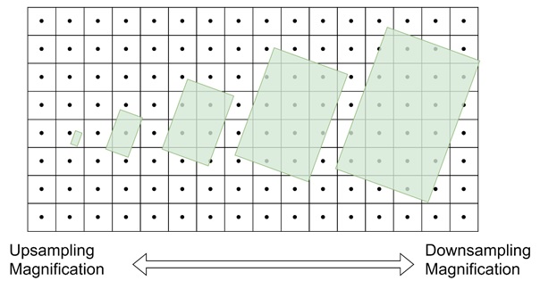
Reconstruction is used when the footprint is smaller than a texel, which means we are magnifying the texture in the image. This process is similar to upsampling an image, where we need to interpolate between texels to produce a smooth result. The most common interpolation technique used in reconstruction is bilinear interpolation.

Bilinear interpolation uses the values of the four nearest texels to compute a smooth color value at any point within the texture. It is a basic reconstruction filter and is effective for reducing blocky artifacts when the texture is magnified. While bilinear interpolation is not the highest-quality filter, it is efficient and often good enough for most applications.

2. Mipmapping

When a pixel footprint is larger than a texel (texture element), we need to compute the average of many texels to prevent aliasing. This is where mipmapping becomes useful. Mipmapping needs creating a sequence of textures. Each at a lower resolution than the original. These lower-resolution textures are called mipmap levels, and they store precomputed averages of the texture over different areas.

The original texture is called the base level, or level 0. Level 1 is generated by downsampling the base level by a factor of 2 in each dimension. This process continues to create as many mipmap levels as needed, with each level representing the texture at a lower resolution. For example, a 1024 x 1024 texture can be downsampled to a 512 x 512 texture for level 1, then to a 256 x 256 texture for level 2, and so on.

When using mipmaps, the appropriate level is chosen based on the size of the pixel footprint. This ensures that the texture is sampled at a resolution that matches the size of the footprint, reducing aliasing without needing to access all the individual texels in the original texture.

Basic Texture Filtering with Mipmaps

To filter mipmaps we can use the simplest way to select a single mipmap level that matches the pixel footprints size. However, since the pixel footprint might not correspond exactly to one mipmap level, we can use linear interpolation between the two closest mipmap levels. This approach is called trilinear filtering.

With trilinear filtering, we first determine the appropriate mipmap level based on the footprint size. If the size falls between two levels, we take samples from both levels and interpolate between them. This results in smoother transitions between mipmap levels. It prevents visual seams or abrupt changes.

Limitations of Mipmapping

Mipmapping is effective at reducing aliasing. But it has limitations. Mipmapping assumes that the pixel footprint is square, but in reality, footprints can be elongated, especially when viewing surfaces at grazing angles. This mismatch causes mipmapping to produce blurred results in one direction. An alternative approach, such as anisotropic filtering, can address this issue by considering the footprints shape more accurately.

Conclusion

In this chapter, we explained the concept of antialiasing texture lookups in texture mapping. We discussed why antialiasing is needed, the role of pixel footprints, and how approximations can help in understanding these footprints.

We then understood two main techniques reconstruction and mipmapping. Reconstruction is useful for magnifying textures, while mipmapping helps in reducing texture details to prevent aliasing.