Window to Viewport Coordinate Transformation

---

---

In the viewing pipeline, we generally see how the model coordinates are transformed to world coordinates and vice versa. The window to viewport coordinate system transformation is needed in every case. This process states that the objects are displayed correctly on the screen while maintaining their relative positioning and proportions.

In this chapter, we will discuss the window to viewport coordinate transformation, explain the reference frames involved, and break down the steps required for this transformation for a better understanding.

Basics of Window and Viewport Coordinate Systems

For understanding this we need a basic recap of window and viewport in computer graphics. As we discussed in the last article that, a window is a rectangular area in the world coordinate system. It defines the part of the scene that we want to display. The window is defined by two points −

• (xw_min, yw_min) − The coordinates of the lower-left corner of the window.
• (xw_max, yw_max) − The coordinates of the upper-right corner of the window.

On the other hand a viewport is the area on the display device (screen) where the image is displayed. The viewport defines how the selected window is mapped to the physical screen. Similar to the window, the viewport is also defined by two points −

• (xv_min, yv_min) − The coordinates of the lower-left corner of the viewport.
• (xv_max, yv_max) − The coordinates of the upper-right corner of the viewport.

When the window and viewport reference frames differ, the transformation process is needed and that states the objects from the window are displayed correctly in the viewport, while maintaining their relative positions and proportions.

Steps to Transform Window Coordinates to Viewport Coordinates

When the window and viewport have different reference frames, we need to follow two main steps to transform the coordinates correctly.

Step 1: Translate the Viewport Origin to the Window Origin

The first step in transforming from window to viewport is to translate the origin of the viewport reference frame to the window reference frame. This means aligning the origins of both coordinate systems.

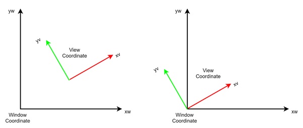
After performing this translation, the new origin of the viewport will coincide with the origin of the window. For example, the (xv, yv) viewport coordinates will align with the (xw, yw) window coordinates.

Step 2: Rotate the Viewport Axis

Once the translation is done, we need to rotate the axes of the viewport to match the window's axes. This ensures that the coordinate axes of the viewport and window are aligned, making it easier to transfer objects from the window to the viewport.

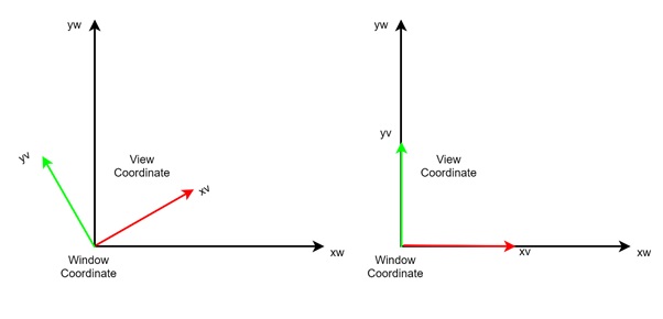
After performing the rotation, both the x and y axes of the window and viewport will be aligned, making the next transformations straightforward. The key here is to maintain the relative positions and proportions of objects during the transformation.

Maintaining Relativity Between Window and Viewport

One of the most critical aspects of transforming window coordinates to viewport coordinates is maintaining the relativity of points. This means ensuring that the relationships between objects and their positions in the window remain unchanged when mapped to the viewport.

For example, if the distance between two points in the window is 10 cm, that relationship should be maintained in the viewport, even if the actual distance is scaled down. The relative positioning of objects should not be disturbed.

Let us say we have an object in the window, and we want to transfer it to the viewport. The object may shrink in size, but the proportional distances between points on the object will remain the same. If the window object has a length of 10 cm and the viewport object has a length of 5 cm, the relativeness of the points is preserved.

Example of Window to Viewport Transformation

Let us consider an example to understand the process in detail.

Suppose we have a window defined by the following coordinates −

$$\mathrm{x_{wmin} \: = \:0,\: \quad y_{wmin} \:=\: 0,\: \quad x_{wmax} \:=\: 100, \quad y_{wmax} \:=\: 100}$$

And the viewport is defined by −

$$\mathrm{x_{vmin} \:=\: 0,\: \quad y_{vmin} \:=\: 0,\: \quad x_{vmax}\: = \:500,\: \quad y_{vmax} \:=\: 500}$$

Transforming a Point

Now, let us say we want to transform a point from the window coordinates (xw, yw) to the viewport coordinates (xv, yv).

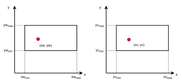
Relative Position in X-Axis

$$\mathrm{\frac{x_v \:-\: x_{wmin}}{x_{wmax} \:-\: x_{wmin}} \:=\: \frac{x_w \:-\: x_{wmin}}{x_{wmax} \:-\: x_{wmin}}}$$

Rearranging the equation, we get −

$$\mathrm{x_v \:=\: x_{wmin} \:+\: \left( \frac{x_w \:-\: x_{wmin}}{x_{wmax} \:-\: x_{wmin}} \right) (x_{wmax} \:-\: x_{wmin})}$$

Then, the similar for y.

Relative Position in Y-Axis

$$\mathrm{\frac{y_v \:-\: y_{vmin}}{y_{vmax} \:-\: y_{vmin}} \:=\: \frac{y_w \:-\: y_{wmin}}{y_{wmax} \:-\: y_{wmin}}}$$

Rearranging the equation, we get −

$$\mathrm{y_v \:=\: y_{vmin} \:+\: \left( \frac{y_w \:-\: y_{wmin}}{y_{wmax} \:-\: y_{wmin}} \right) (y_{vmax} \:-\: y_{vmin})}$$

These equations ensure that the points are mapped correctly from the window to the viewport.

Scaling Factors

To simplify the process, we introduce scaling factors −

$$\mathrm{s_x \:=\: \frac{x_w \:-\: x_{wmin}}{x_{wmax} \:-\: x_{wmin}}}$$

$$\mathrm{s_y \:=\: \frac{y_w \:-\: y_{wmin}}{y_{wmax} \:-\: y_{wmin}}}$$

The scaling factors help in determining the transformation of points. If s_x = s_y, it means that both the x and y coordinates are transformed equally, preserving the aspect ratio. However, if s_x ≠ s_y, the transformation might result in either stretching or compressing the objects.

In this case, since xv_max = 500 and xw_max = 100, the scaling factor for x would be −

$$\mathrm{s_x \:=\: \frac{500 \:-\: 0}{100 \:-\: 0} \:=\: 5}$$

Similarly, for the y-axis −

$$\mathrm{s_y \:=\: \frac{500 \:-\: 0}{100 \:-\: 0} \:=\: 5}$$

Since s_x = s_y, the transformation will maintain the aspect ratio of the objects. Whatever is present in the window will appear the same in the viewport, just scaled up by a factor of 5.

Example of Calculation

Let us transform a point (50, 50) from the window to the viewport −

For the x-coordinate −

$$\mathrm{x_v \:=\: 0 \:+\: \frac{50 \:-\: 0}{100 \:-\: 0}\: \times \:(500 \:-\: 0)}$$

$$\mathrm{x_v \:=\: 250}$$

For the y-coordinate −

$$\mathrm{y_v \:=\: 0 \:+\: \frac{50 \:-\: 0}{100 \:-\: 0} \:\times \:(500 \:-\: 0)}$$

$$\mathrm{y_v \:=\: 250}$$

Thus, the point (50, 50) in the window maps to (250, 250) in the viewport.

Conclusion

In this chapter, we discussed the Window to Viewport Coordinate Transformation in computer graphics. We also seen the basic definitions of window and viewport, how their reference frames can differ, and the two primary steps involved in transforming coordinates: translation and rotation.

We also covered the importance of maintaining the relativity of points between the window and viewport. Finally, we walked through a detailed example to show how the transformation equations are applied in practice for a detailed understanding.